Modular Multiplicative Inverse

This post is a pre-requisite for the next thing I want to talk about so may not make a whole lot of sense or be all that interesting until shown in that context.

Say you have a function like this:

(a*x) \mod m = n

If you know the values of a, m and n, how do you solve for x? Note in this post we are only dealing with integers, so we are looking for the integer solution for x.

It might be hard to visualize with so many symbols, so here it is with some constants:

(5*x) \mod 7 = 3

How would you solve that for x? In other words, what do you need to multiply 5 by, so that when you divide the result by 7, that you get 3 as the remainder?

One way to solve for x would be brute force. We could try plugging every value from 0 to 6 into x (every value from 0 to n-1), and see if any gives us the result we are looking for.

Brute force can be a challenge if the numbers are really large, like in some cryptographic situations.

Interestingly, there might not even be a valid answer for x that satisfies the equation! The below has no answer for instance:

(2*x) \mod 8 = 5

Better Than Brute Force

There’s something called the “Modular Multiplicative Inverse” which looks eerily familiar:

(a*x) \mod m = 1

Where a and m are known, and the inverse itself is the value of x.

Using the same constants we did above, that gives us this:

(5*x) \mod 7 = 1

In this case, the inverse (x) is 3. You can verify that by seeing that (5*3) % 7 is 1.

Once you have the inverse, if you wanted to solve the original equation where the modulus end up being 3, you just multiply the inverse by the desired modulus amount. Since the inverse is 3 and the desired modulus value is 3, you multiply them together and get 9. Plugging the numbers in, we can see that (5*9) % 7 = 3.

Pretty cool, but how to calculate the inverse? You can calculate it by using something called the “Extended Euclidean Algorithm”.

The regular Euclidean algorithm is in a post here: Programmatically Calculating GCD and LCM.

The extended euclidean algorithm is explained really well on wikipedia: Wikipedia: Extended Euclidean Algorithm.

Sample Code

Here’s some sample code that asks the user for input and solves these style of equations for x. Below the code I’ll show some example runs and talk about a few more things.

#include <stdio.h>
#include <algorithm>
#include <array>

//=================================================================================
unsigned int ExtendedEuclidianAlgorithm (int smaller, int larger, int &s, int &t)
{
    // make sure A <= B before starting
    bool swapped = false;
    if (larger < smaller)
    {
        swapped = true;
        std::swap(smaller, larger);
    }

    // set up our storage for the loop.  We only need the last two values so will
    // just use a 2 entry circular buffer for each data item
    std::array<int, 2> remainders = { larger, smaller };
    std::array<int, 2> ss = { 1, 0 };
    std::array<int, 2> ts = { 0, 1 };
    int indexNeg2 = 0;
    int indexNeg1 = 1;

    // loop
    while (1)
    {
        // calculate our new quotient and remainder
        int newQuotient = remainders[indexNeg2] / remainders[indexNeg1];
        int newRemainder = remainders[indexNeg2] - newQuotient * remainders[indexNeg1];

        // if our remainder is zero we are done.
        if (newRemainder == 0)
        {
            // return our s and t values as well as the quotient as the GCD
            s = ss[indexNeg1];
            t = ts[indexNeg1];
            if (swapped)
                std::swap(s, t);
            return remainders[indexNeg1];
        }

        // calculate this round's s and t
        int newS = ss[indexNeg2] - newQuotient * ss[indexNeg1];
        int newT = ts[indexNeg2] - newQuotient * ts[indexNeg1];

        // store our values for the next iteration
        remainders[indexNeg2] = newRemainder;
        ss[indexNeg2] = newS;
        ts[indexNeg2] = newT;

        // move to the next iteration
        std::swap(indexNeg1, indexNeg2);
    }
}

//=================================================================================
void WaitForEnter ()
{
    printf("nPress Enter to quit");
    fflush(stdin);
    getchar();
}

//=================================================================================
int main(int argc, char **argv)
{
    // get user input
    int a, m, n;
    printf("Given a, m and n, solves for X.n(a * X) %% m = nnn");
    printf("a = ");
    scanf("%i", &a);
    printf("m = ");
    scanf("%i", &m);
    printf("n = ");
    scanf("%i", &n);

    // show details of what they entered
    printf("n(%i * X) mod %i = %in", a, m, n);

    // Attempt brute force
    printf("nBrute Force Testing X from 0 to %i:n", (m-1));
    for (int i = 0; i < m; ++i) {
        if ((a*i) % m == n)
        {
            printf("  X = %in", i);
            printf("  %i mod %i = %in", a*i, m, (a*i) % m);
            break;
        }
        else if (i == (m - 1))
        {
            printf("  No solution!n");
        }
    }

    // Attempt inverse via Extended Euclidean Algorithm
    printf("nExtended Euclidean Algorithm:n");
    int s, t;
    int GCD = ExtendedEuclidianAlgorithm(a, m, s, t);

    // report failure if we couldn't do inverse
    if (GCD != 1)
    {
        printf("  Values are not co-prime, cannot invert! GCD = %in", GCD);
    }
    // Else report details of inverse and show that it worked
    else
    {
        printf("  Inverse = %in", t);
        printf("  X = Inverse * n = %in", t*n);
        printf("  %i mod %i = %in", a*t*n, m, (a*t*n) % m);
    }

    WaitForEnter();
    return 0;
}

Example Runs

Here is a normal run that solves (7*x) \mod 9 = 2, to come up with a value of 8 for x.

Here is a run that solves (5*x) \mod 7 = 3. Brute force gives us a value of 2 for x, while the inverse gives us a value of 9. Both are valid, and in fact are equivalent since 9 % 7 = 2. This shows that getting the inverse and then multiplying it to get the desired answer doesn’t always give you the smallest possible value of x.

Here is a large number run that solves (7*x) \mod 1000001 = 538. Brute force gives a value of 571,506 for x, while using the inversion method gives us a value of 230,571,736.

Lastly, here is a run that solves (8*x) \mod 6 = 4. Brute force gives us a value of 2 for x, but interestingly, it isn’t invertible, so the inversion based solution can’t even find us an answer!

This happens when a and m are not co-prime. In other words, if they have a GCD that isn’t 1, they aren’t coprime, and the modulus can’t be inverted.

Links

You can read more about the modular multiplicative inverse here: Wikipedia: Modular Multiplicative Inverse.

Improving the Security of the Super Simple Symmetric Leveled Homomorphic Encryption Implementation

The last post showed a super simple encryption algorithm that let an untrusted person perform calculations with encrypted data such that when they gave the results back to you, you could decrypt them and get the results of the calculation as if they were done on the unencrypted values. The best part was that this untrusted party had no knowledge of the data it was doing the calculations on.

While it was (hopefully) easy to understand, there were a lot of problems with it’s security. The biggest of which probably was the fact that the encryption of a false bit was the secret key itself!

This post is going to slightly increase the complexity of the encryption operation to match what the paper that I’m getting this stuff from says to do (Fully Homomorphic Encryption over the Integers).

All of the other operations – like XOR, AND, Decryption, use of constants – remain the same. It’s just the process of turning a plain text bit into a cipher text bit that is going to change.

Disclaimer: I am a game programmer, not a cryptographer, and you should REALLY do your own investigation and consult experts before actually rolling anything out to production or trusting that what I say is correct!

Improvement #1 – Multiply Key By Random Number

The scheme to encrypt a plaintext bit from the last blog post was this:

encryptedBit = key + value ? 1 : 0;

A major problem with that scheme is that if you encrypt a false bit, you get the key itself.

Another problem that we touched on was that the parity of the plain text bit (whether it was odd or even, aka a 1 or a 0) was always opposite of the parity of the cipher text.

Yet another problem was that for the same key, 0 always encrypted to the same value, and 1 always encrypted to the same value, which was the “0” encrypted value, plus 1.

We are going to address all of these problems by adding a simple operation to encryption. We are just going to multiply the key by a random number before adding the plain text bit in. That gives us the following:

encryptedBit = key*randomNumber + value ? 1 : 0;

Where randomNumber is at least 1.

This above helps in the following ways:

  • Encrypting false doesn’t always just give you the key anymore!
  • Since the cipherBit divided by the key is now a random number (and since the key is an odd number), it will be random whether the parity of the cipher text matches or mismatches the plain text. You can no longer use that information to figure out the value of the encrypted bit!
  • If you encrypt a false value, you will get different values each time. Same when encrypting a true value. When looking at two ciphertexts that have the same underlying plaintext value, you will no longer be able to tell that they are equal just by looking at them, or be able to tell that one is larger than the other so must be the true bit!

That is a pretty good improvement, but we can do a little better.

Improvement #2 – Add Random Noise

The second improvement we are going to do is add random noise to our encrypted value. This will make it so encrypting a false bit will not result in a multiple of the key, but will instead result in NEARLY a multiple of the key, which is a harder problem to figure out as an attacker.

You might ask how we are going to preserve our encrypted value if we are adding random noise into the result. Well, in actuality, all we really need to preserve is the lowest bit, so we are going to add an EVEN NUMBERED amount of noise.

That makes our encryption scheme become this:

encryptedBit = key*randomNumber1 + 2*randomNumber2 + value ? 1 : 0;

While this increases our security, it also increases the noise (error) in our encrypted data, which makes it so we can do fewer operations before the error gets too large and we start getting wrong answers.

There we are, our encryption scheme now matches the one described in the paper. All the rest of our operations remain unchanged.

Security

The above looks good, but what range of values should be we use for randomNumber1 and randomNumber2 and the actual size of the key?

The paper refers to a security parameter lambda (\lambda) that everything else is based on.

It says that the size of the key (N) should be (\lambda^2) bits, randomNumber1 should be around 2^{N^3} (N^3 bits) and that randomNumber2 should be around 2^{\sqrt{N}} (\sqrt{N} bits).

It also says that the best known attack against this algorithm takes about 2^{N^2} operations and that you can assume an attacker is going to be able to do a billion operations per second (per this info here). Note that 1 billion operations per second is a typical computer, not a super computer or a distributed attack using a bot network!

Let’s look at some example values for lambda!

Lambda Key Size RN1 Size RN2 Size Attack Time
80 800B 30.5GB 10B 38 million years
60 450B 5.4GB 8B 36 years
40 200B 488MB 5B 17 minutes
20 50B 7.6MB 3B < 1 second

Ouch! RandomNumber1 sure is huge isn’t it? I’ve double and tripple checked and that really does seem to be correct. Encrypting a single bit is essentially going to be as large as RandomNumber1. That is so unwieldy it’s ridiculous. I’m going to quadruple check that I think because that is just insane…

BTW quick tangent. An interesting thing to note is that if your key is an even number, instead of an odd number, noise/error can grow as much as it wants, and will never give you the wrong result! That means that by using an even numbered key, this scheme is fully homomorphic. However, using an even key, encryptedBit % 2 == decryptedBit, so it’s super insecure.

I’ve been thinking about it quite a bit, but I can’t think of any avenues to use an even numbered key but still have any semblance of real security. If you can think of a way, go publish a paper about it and become famous! 😛

Example Code

Here is some sample code from last post with the new encryption routine. I had to decrease the number of bits in the addition tests, and I had to tone down the security quite a bit to make it fit within 64 bits.

#include <stdio.h>
#include <stdint.h>
#include <random>
#include <array>
#include <inttypes.h>

typedef uint64_t uint64;

// Increase this value to increase the size of the key, and also the maximum
// size of the error allowed.
// If you set it too high, operations will fail when they run out of storage space
// in the 64 bit ints.  If you set it too low, you will not be able to do very many
// operations in a row.
// The recomended values for good security for these numbers are way too large to
// fit in a uint64, so adjusting them down to show their effects while using uint64s
const size_t c_numKeyBits = 15;
const size_t c_numNoiseBits = 3; //size_t(sqrt(c_numKeyBits));
const size_t c_numMultiplierBits = 4; //c_numKeyBits * c_numKeyBits * c_numKeyBits;

#define Assert(x) if (!(x)) ((int*)nullptr)[0] = 0;

//=================================================================================
// TODO: Replace with something crypto secure if desired!
uint64 RandomUint64 (uint64 min, uint64 max)
{
    static std::random_device rd;
    static std::mt19937 gen(rd());
    std::uniform_int_distribution<uint64> dis(min, max);
    return dis(gen);
}

//=================================================================================
void WaitForEnter ()
{
    printf("Press Enter to quit");
    fflush(stdin);
    getchar();
}

//=================================================================================
uint64 GenerateKey ()
{
    // Generate an odd random number in [2^(N-1), 2^N)
    // N is the number of bits in our key
    // The key also defines the maximum amount of error allowed, and thus the number
    // of operations allowed in a row.
    uint64 key = RandomUint64(0, (uint64(1) << uint64(c_numKeyBits)) - 1);
    key = key | (uint64(1) << uint64(c_numKeyBits - 1));
    key = key | 1;
    return key;
}

//=================================================================================
bool Decrypt (uint64 key, uint64 value)
{
    return ((value % key) % 2) == 1;
}

//=================================================================================
uint64 Encrypt (uint64 key, bool value)
{
    uint64 keyMultiplier = RandomUint64(0, (1 << c_numMultiplierBits) - 2) + 1;
    uint64 noise = RandomUint64(0, (1 << c_numNoiseBits) - 1);
    uint64 ret = key * keyMultiplier + 2 * noise + (value ? 1 : 0);
    Assert(Decrypt(key, ret) == value);
    return ret;
}

//=================================================================================
uint64 XOR (uint64 A, uint64 B)
{
    return A + B;
}

//=================================================================================
uint64 AND (uint64 A, uint64 B)
{
    return A * B;
}

//=================================================================================
float GetErrorPercent (uint64 key, uint64 value)
{
    // Returns what % of maximum error this value has in it.  When error >= 100%
    // then we have hit our limit and start getting wrong answers.
    return 100.0f * float(value % key) / float(key);
}

//=================================================================================
uint64 FullAdder (uint64 A, uint64 B, uint64 &carryBit)
{
    // homomorphically add the encrypted bits A and B
    // return the single bit sum, and put the carry bit into carryBit
    // From http://en.wikipedia.org/w/index.php?title=Adder_(electronics)&oldid=381607326#Full_adder
    uint64 sumBit = XOR(XOR(A, B), carryBit);
    carryBit = XOR(AND(A, B), AND(carryBit, XOR(A, B)));
    return sumBit;
}

//=================================================================================
int main (int argc, char **argv)
{
    // run this test a bunch to show that it works.  If you get a divide by zero
    // in an Assert, that means that it failed, and hopefully it's because you
    // increased c_numKeyBits to be too large!
    printf("Verifying 10000 truth tables.  Details of first one:n");
    for (int index = 0; index < 10000; ++index)
    {
        // make our key and a true and false bit
        uint64 key = GenerateKey();
        uint64 falseBit1 = Encrypt(key, false);
        uint64 falseBit2 = Encrypt(key, false);
        uint64 trueBit1  = Encrypt(key, true);
        uint64 trueBit2  = Encrypt(key, true);

        // report the results for the first iteration of the loop
        if (index == 0)
        {
            printf("Key 0x%" PRIx64 ", false = 0x%" PRIx64 ", 0x%" PRIx64 " true = 0x%" PRIx64 " 0x%" PRIx64 "n", key, falseBit1, falseBit2, trueBit1, trueBit2);
            printf("  [0 xor 0] = 0   0x%" PRIx64 " xor(+) 0x%" PRIx64 " = 0x%" PRIx64 " (%i err=%0.2f%%)n", falseBit1, falseBit2, XOR(falseBit1, falseBit2), Decrypt(key, XOR(falseBit1, falseBit2)) ? 1 : 0, GetErrorPercent(key, XOR(falseBit1, falseBit2)));
            printf("  [0 xor 1] = 1   0x%" PRIx64 " xor(+) 0x%" PRIx64 " = 0x%" PRIx64 " (%i err=%0.2f%%)n", falseBit1, trueBit2 , XOR(falseBit1, trueBit2 ), Decrypt(key, XOR(falseBit1, trueBit2 )) ? 1 : 0, GetErrorPercent(key, XOR(falseBit1, trueBit2 )));
            printf("  [1 xor 0] = 1   0x%" PRIx64 " xor(+) 0x%" PRIx64 " = 0x%" PRIx64 " (%i err=%0.2f%%)n", trueBit1 , falseBit2, XOR(trueBit1 , falseBit2), Decrypt(key, XOR(trueBit1 , falseBit2)) ? 1 : 0, GetErrorPercent(key, XOR(trueBit1 , falseBit2)));
            printf("  [1 xor 1] = 0   0x%" PRIx64 " xor(+) 0x%" PRIx64 " = 0x%" PRIx64 " (%i err=%0.2f%%)n", trueBit1 , trueBit2 , XOR(trueBit1 , trueBit2 ), Decrypt(key, XOR(trueBit1 , trueBit2 )) ? 1 : 0, GetErrorPercent(key, XOR(trueBit1 , trueBit2 )));
            printf("  [0 and 0] = 0   0x%" PRIx64 " and(*) 0x%" PRIx64 " = 0x%" PRIx64 " (%i err=%0.2f%%)n", falseBit1, falseBit2, AND(falseBit1, falseBit2), Decrypt(key, AND(falseBit1, falseBit2)) ? 1 : 0, GetErrorPercent(key, XOR(falseBit1, falseBit2)));
            printf("  [0 and 1] = 0   0x%" PRIx64 " and(*) 0x%" PRIx64 " = 0x%" PRIx64 " (%i err=%0.2f%%)n", falseBit1, trueBit2 , AND(falseBit1, trueBit2 ), Decrypt(key, AND(falseBit1, trueBit2 )) ? 1 : 0, GetErrorPercent(key, XOR(falseBit1, trueBit2 )));
            printf("  [1 and 0] = 0   0x%" PRIx64 " and(*) 0x%" PRIx64 " = 0x%" PRIx64 " (%i err=%0.2f%%)n", trueBit1 , falseBit2, AND(trueBit1 , falseBit2), Decrypt(key, AND(trueBit1 , falseBit2)) ? 1 : 0, GetErrorPercent(key, XOR(trueBit1 , falseBit2)));
            printf("  [1 and 1] = 1   0x%" PRIx64 " and(*) 0x%" PRIx64 " = 0x%" PRIx64 " (%i err=%0.2f%%)n", trueBit1 , trueBit2 , AND(trueBit1 , trueBit2 ), Decrypt(key, AND(trueBit1 , trueBit2 )) ? 1 : 0, GetErrorPercent(key, XOR(trueBit1 , trueBit2 )));
        }

        // Verify truth tables for XOR and AND
        Assert(Decrypt(key, XOR(falseBit1, falseBit2)) == false);
        Assert(Decrypt(key, XOR(falseBit1, trueBit2 )) == true );
        Assert(Decrypt(key, XOR(trueBit1 , falseBit2)) == true );
        Assert(Decrypt(key, XOR(trueBit1 , trueBit2 )) == false);

        Assert(Decrypt(key, AND(falseBit1, falseBit2)) == false);
        Assert(Decrypt(key, AND(falseBit1, trueBit2 )) == false);
        Assert(Decrypt(key, AND(trueBit1 , falseBit2)) == false);
        Assert(Decrypt(key, AND(trueBit1 , trueBit2 )) == true );
    }

    // Do multi bit addition as an example of using compound circuits to
    // do meaningful work.
    const size_t c_numBitsAdded = 3;
    printf("nDoing 10000 Multibit Additions.  Details of first one:n");
    std::array<uint64, c_numBitsAdded> numberAEncrypted;
    std::array<uint64, c_numBitsAdded> numberBEncrypted;
    std::array<uint64, c_numBitsAdded> resultEncrypted;
    std::array<uint64, c_numBitsAdded> carryEncrypted;
    for (int index = 0; index < 10000; ++index)
    {
        // generate the numbers we want to add
        uint64 numberA = RandomUint64(0, (1 << c_numBitsAdded) - 1);
        uint64 numberB = RandomUint64(0, (1 << c_numBitsAdded) - 1);

        // generate our key
        uint64 key = GenerateKey();

        // encrypt our bits
        for (int bitIndex = 0; bitIndex < c_numBitsAdded; ++bitIndex)
        {
            numberAEncrypted[bitIndex] = Encrypt(key, (numberA & (uint64(1) << uint64(bitIndex))) != 0);
            numberBEncrypted[bitIndex] = Encrypt(key, (numberB & (uint64(1) << uint64(bitIndex))) != 0);
        }

        // do our multi bit addition!
        // we could initialize the carry bit to 0 or the encrypted value of 0. either one works since 0 and 1
        // are also poor encryptions of 0 and 1 in this scheme!
        uint64 carryBit = Encrypt(key, false);
        for (int bitIndex = 0; bitIndex < c_numBitsAdded; ++bitIndex)
        {
            carryEncrypted[bitIndex] = carryBit;
            resultEncrypted[bitIndex] = FullAdder(numberAEncrypted[bitIndex], numberBEncrypted[bitIndex], carryBit);
        }

        // decrypt our result
        uint64 resultDecrypted = 0;
        for (int bitIndex = 0; bitIndex < c_numBitsAdded; ++bitIndex)
        {
            if (Decrypt(key, resultEncrypted[bitIndex]))
                resultDecrypted |= uint64(1) << uint64(bitIndex);
        }

        // report the results for the first iteration of the loop
        if (index == 0)
        {
            printf("Key 0x%" PRIx64 ", %" PRId64 " + %" PRId64 " in %i bits = %" PRId64 "n", key, numberA, numberB, c_numBitsAdded, (numberA + numberB) % (1 << c_numBitsAdded));
            for (int bitIndex = 0; bitIndex < c_numBitsAdded; ++bitIndex)
                printf("  A[%i] = 0x%" PRIx64 " (%i err=%0.2f%%)n", bitIndex, numberAEncrypted[bitIndex], Decrypt(key, numberAEncrypted[bitIndex]), GetErrorPercent(key, numberAEncrypted[bitIndex]));
            printf("+n");
            for (int bitIndex = 0; bitIndex < c_numBitsAdded; ++bitIndex)
                printf("  B[%i] = 0x%" PRIx64 " (%i err=%0.2f%%)n", bitIndex, numberBEncrypted[bitIndex], Decrypt(key, numberBEncrypted[bitIndex]), GetErrorPercent(key, numberBEncrypted[bitIndex]));
            printf("=n");
            for (int bitIndex = 0; bitIndex < c_numBitsAdded; ++bitIndex)
                printf("  Result[%i] = 0x%" PRIx64 " (%i err=%0.2f%%)n", bitIndex, resultEncrypted[bitIndex], Decrypt(key, resultEncrypted[bitIndex]), GetErrorPercent(key, resultEncrypted[bitIndex]));
            printf("Carry Bits =n");
            for (int bitIndex = 0; bitIndex < c_numBitsAdded; ++bitIndex)
                printf("  Result[%i] = 0x%" PRIx64 " (%i err=%0.2f%%)n", bitIndex, carryEncrypted[bitIndex], Decrypt(key, carryEncrypted[bitIndex]), GetErrorPercent(key, carryEncrypted[bitIndex]));
            printf("result decrypted = %" PRId64 "n", resultDecrypted);
        }

        // make sure that the results match, keeping in mind that the 4 bit encryption may have rolled over
        Assert(resultDecrypted == ((numberA + numberB) % (1 << c_numBitsAdded)));
    }

    WaitForEnter();
    return 0;
}

Here’s the output of an example run.

Links

Another paper about symmetric HE over the integers: Symmetric Somewhat Homomorphic Encryption over the Integers

An implementation of FHE: Implementation of the DGHV fully homomorphic encryption scheme

Next Up

Here are some interesting avenues to explore with this stuff. More blog posts coming in the future about these topics, but for now, here they are in case you want to check them out yourself:

  • Making the public / private key implementation
  • Make this stuff work with multi precision math to be able to make realistically sized and see what sort of perf it gives
  • Show how to achieve fully homomorphic encryption using boot strapping and/or modulus switching
  • Further explore tuning down security parameters to get game quality HE
  • Explore the other known methods for implementing HE. HE over the integers is apparently very easy to understand compared to other methods, but other methods may have different characteristics – like maybe not being crazy gigantic

Super Simple Symmetric Leveled Homomorphic Encryption Implementation

Homomorphic encryption is a pretty interesting thing. It allows you to do calculations on encrypted data such that when you decrypt the results, it’s as if you did the calculations on the unencrypted data. This allows computation to happen without the person doing the computation knowing what the data actually is!

Brief History

For a long time, cryptographers wondered if fully homomorphic encryption was even possible. There were various encryption algorithms that could perform SOME operations homomorphically (RSA can do multiplication for instance!), but there weren’t any that could do ALL operations. In other words, you couldn’t execute arbitrary computations.

Those types of algorithms are called “Partially Homomorphic Encryption” or PHE.

Another problem standing in the way of fully homomorphic encryption was that many algorithms would only have a limited count of operations they could perform before error would accumulate and they would start giving incorrect answers. In essence they were limited to evaluating low degree polynomials.

Those types of algorithms are called “Somewhat Homomorphic Encryption” or SWHE.

In contrast, Fully Homomorphic Encryption (FHE) can perform an unlimited number of homomorphic operations, and it can perform any operation homomorphically. It is unbounded in both ways.

Amazingly, In 2009 Craig Gentry figured out the first fully homomorphic encryption scheme! With his setup, you can calculate both XOR and AND on encrypted bits, which makes it Turing complete. It is also able to keep errors from becoming too large by using an ingenious bootstrapping technique to decrease accumulated error. Here’s a link to his PHd thesis: A Fully Homomorphic Encryption Scheme.

Unfortunately, the current implementations of secure FHE take too much computational power to be practical in most situations – like 30 minutes to calculate an AND between 2 bits!

In this post I’m going to show you a super simple HE implementation that will be very easy to understand. It won’t be fully homomorphic, but it will be “leveled” (or, somewhat homomorphic), meaning it is Turing complete, but the count of calculations you can perform are limited due to error creeping in. It also won’t be secure – due to making it easy to understand – but it will be lightning fast.

This will be a symmetric key algorithm, but as we’ll explore in future posts, it can also be used for public key algorithms.

Why Is HE Useful?

One thing you could do with HE is store your financial transactions encrypted on a server. The server could run queries and calculations on your financial data and send back the results. You could then unencrypt the result and see what the values are, even though the server itself – which generated the values – has no idea what the numbers actually are.

Another use could be in games. Whether you are playing a first person shooter, or a real time strategy game, many different types of games send information about each player to every other player in the game. Hashes of game state can be used to make sure that everyone is in agreement about calculations to prevent a player from cheating by WRITING to a value they shouldn’t be writing to (or, at least you can detect when they do, and use majority rule to boot them out of the game), but how do you stop a player from READING a value they shouldn’t be reading?

Using HE, you could encrypt the data you need to send to players that they shouldn’t be able to read. With this, they could still do game play logic calculations on the data, and calculate hashes of the encrypted results to ensure that all players were in agreement, but with HE, they wouldn’t gain knowledge of the data they were working with.

In other words, player A could verify that player B’s state is correct and they haven’t cheated, without player A getting details about player B’s state.

In theory this could eliminate or at least help combat things like wall hacks and other “data read” based cheats. In practice there would be some complications to work out, even if it wasn’t crazy slow to calculate, but the fact that there is a path to addressing these issues is pretty exciting! People are working on improving speed, and games don’t need the same level of security that other usage cases do.

How To Do It

Here are the details of this super simple leveled homomorphic symmetric key algorithm.

By the way, all the percent signs below mean “modulus” which is just the remainder of a division. 25 % 4 = 1 for instance, because 25/4 = 6 with a remainder of 1. That remainder of 1 is what we get when we take the modulus. A term you’ll see more often if reading through this stuff on your own will be “residue”. Don’t let that word scare you, it is just another name for the remainder.

Making A Secret Key

To make a key, generate an odd random number between 2^(N-1) and 2^N. In other words, it will be N random bits, except the highest and lowest bit will be set to 1. N is the size of your secret key. Larger keys are more secure, and allow more computations to be done in a row, but they also take more storage space. If you are using a fixed size int – like say a uint32 – a larger key will make you run out of those 32 bits sooner.

key = RandomNumber(0, (1 << N) - 1) | 1 | (1 << (N - 1));

Encrypt

To encrypt a bit, the encrypted value is just the key plus the value of the unencrypted bit (0 or 1).

encryptedBit = key + value ? 1 : 0;

Decrypt

To decrypt a bit, you take the encrypted bit modulo the key, and then modulo 2.

decryptedBit = (encryptedBit % key) % 2;

XOR

To do an XOR of two encrypted bits, you just add the two values together.

xorResult = encryptedBit1 + encryptedBit2;

AND

To do an AND of two encrypted bits, you just multiply the two values together.

andResult = encryptedBit1 * encryptedBit2;

Example

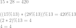
Let’s run through an example to see this in action.

We’ll use a 4 bit key, and say that the key is 13 (1101 in binary).

Let’s encrypt some bits:

trueBitEncrypted = key + 1 = 13 + 1 = 14 \newline falseBitEncrypted = key + 0 = 13 + 0 = 13

Let’s do some logical operations:

Xor00 = falseBitEncrypted + falseBitEncrypted = 13 + 13 = 26 \newline Xor01 = falseBitEncrypted + trueBitEncrypted  = 13 + 14 = 27 \newline Xor10 = trueBitEncrypted  + falseBitEncrypted = 14 + 13 = 27 \newline Xor11 = trueBitEncrypted  + trueBitEncrypted  = 14 + 14 = 28 \newline \newline And00 = falseBitEncrypted * falseBitEncrypted = 13 * 13 = 169 \newline And01 = falseBitEncrypted * trueBitEncrypted  = 13 * 14 = 182 \newline And10 = trueBitEncrypted  * falseBitEncrypted = 14 * 13 = 182 \newline And11 = trueBitEncrypted  * trueBitEncrypted  = 14 * 14 = 196 \newline \newline FalseXorFalseAndTrue = falseBitEncrypted + falseBitEncrypted * trueBitEncrypted = 13 + 13 * 14 = 195

Notice how AND is a multiplication where XOR is an addition, and that the result of an AND operation is a larger number than an XOR operation. This means that if you are working with a specific sized number (again, such as a uint32), that you can do fewer ANDs than XORs before you run out of bits. When you run out of bits and your number has integer overflow, you have hit the cieling of this leveled HE scheme. That means that ANDs are more expensive than XORs when considering the number of computations you can do.

Ok, time to decrypt our XOR values!

Xor00Decrypted = ((Xor00 \% key) \% 2) = (26 \% 13) \% 2 = 0 \newline Xor01Decrypted = ((Xor01 \% key) \% 2) = (27 \% 13) \% 2 = 1 \newline Xor10Decrypted = ((Xor10 \% key) \% 2) = (27 \% 13) \% 2 = 1 \newline Xor11Decrypted = ((Xor11 \% key) \% 2) = (28 \% 13) \% 2 = 0 \newline

XOR is looking correct, how about AND?

And00Decrypted = ((And00 \% key) \% 2) = (169 \% 13) \% 2 = 0 \newline And01Decrypted = ((And01 \% key) \% 2) = (182 \% 13) \% 2 = 0 \newline And10Decrypted = ((And10 \% key) \% 2) = (182 \% 13) \% 2 = 0 \newline And11Decrypted = ((And11 \% key) \% 2) = (196 \% 13) \% 2 = 1 \newline

AND is looking good as well. Lastly let’s decrypt the compound operation:

FalseXorFalseAndTrueDecrypted = ((FalseXorFalseAndTrue \% key) \% 2) = (195 \% 13) \% 2 = 0

Lookin good!

Intuition

Let’s get some intuition for why this works…

Key Generation

First up, why is it that the key needs to have it’s high bit set? Well, on one hand, larger keys are more secure, and allow more room for error accumulation so allow more operations to be done. On the other hand, this is kind of misleading to say. If you generate ANY random odd integer, there will be a highest bit set to 1 SOMEWHERE. You technically don’t need to store the zeros above that. So i guess you could look at it like you are just generating ANY random odd integer, and you could figure out N FROM that value (the position of the highest bit). Thinking about it the way we do though, it lets us specify how many bits we actually want to commit to for the key which gives us more consistent behavior, upper bound storage space, etc.

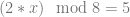
Secondly, why does the key need to be odd?

Let’s say that you have two numbers A and B where A represents an encrypted bit and B represents the encryption key. If B is even, then A % B will always have the same parity (whether it’s even or odd) as A. Since we are trying to hide whether our encrypted bit is 0 or 1 (even or odd), that makes it very bad encryption since you can recover the plain text bit by doing encryptedValue % 2. If on the other hand, B is odd, A % B will have the same parity as A only if A / B is even.

This doesn’t really make much of a difference in the scheme in this post, because A / B will always be 1 (since the encrypted bit is the key plus the plain text bit), but in the next scheme it is more important because A / B will be a random number, which means that it will be random with a 50/50 chance whether or not the parity of the encrypted bit matches the parity of the plain text bit. Since it’s an even chance whether it matches or not, that means that an attacker can’t use that information to their advantage.

While it’s true that when generating a random key, there is a 50/50 chance of whether you will get an even or odd key, you can see how we’d be in a situation where 75% of the time the parity of the ciphertext would match the parity of the plaintext if we allowed both even and off keys.

That would mean that while an attacker couldn’t know for CERTAIN whether an encrypted bit is 1 or 0 based on the cipher text, they can guess with 75% confidence that the unencrypted bit will just be the cipher text % 2, which is no good! So, we are better off sticking with an odd numbered key in this scheme. But again, that won’t really matter until the next post!

XOR as Addition

I know that I’m going to butcher this explanation a bit in the eyes of someone who knows this math stuff better than me. If you are reading this and see that I have indeed done that, please drop me a line or leave a comment and let me know what I’ve missed or could explain better. I suspect there’s something about rings going on here (;

Believe it or not, when you add two numbers together and then take the modulus, you get the same answer as if you did the modulus on the two numbers, added them together, and then took the modulus again.

In other words, adding two numbers can be seen as adding their residue (remainder).

Let me show you an example.

15 + 28 = 43 \newline \newline ((15 \% 13) + (28 \% 13)) \% 13 = 43 \% 13 \newline (2 + 2) \% 13 = 4 \newline 4 = 4

Let’s try another one. I’m picking these numbers “randomly” out of my head 😛

28 + 47 = 75 \newline \newline ((28 \% 8) + (47 \% 8)) \% 8 = 75 \% 8 \newline (4 + 7) \% 8 = 3 \newline 3 = 3

OK makes sense, but who cares about that?

Well, believe it or not, 1 bit addition is the same as XOR! This means that you can add numbers together, which adds the modulus of their key together, which then in turn adds that number mod 2 together, to preserve the encrypted parity (odd or even-ness).

Check out this 2 bit binary math. Keep in mind that with 1 bit results, you would only keep the right most binary digit. I’m showing two digits to show you that it is in fact binary addition, and that the right most bit is in fact the same as XOR.

0 + 0 = 00 \newline 0 + 1 = 01 \newline 1 + 0 = 01 \newline 1 + 1 = 10

One thing to note before we move on is that since we are doing a modulus against the key, when the remainder gets to be too large it rolls over. When it rolls over, we start getting the wrong answers and have hit our ceiling of how many operations we can do. So, our encrypted value modulo the key divided by the key can be seen as where we are at by percentage towards our error ceiling.

To avoid hitting the problem of error getting too high too quickly and limiting your calculation count too much you can increase the key size. When you do that you’ll then run out of bits in your fixed size integer storage faster. To avoid THAT problem you can use “multi precision math libraries” to allow your integers to use an arbitrary number of bytes. This is what many real crypto algorithms use when they need to deal with very large numbers.

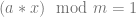
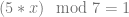
AND as Multiplication

Similar to the above, when you multiply two numbers and take a modulus of the result, it’s the same as if you took the modulus of the two numbers, multiplied that, and then took the modulus of the result.

In other words, when you multiply two numbers, you can think of it as also multiplying their residue (remainder).

Using the first example numbers from above:

15 * 28 = 420 \newline \newline ((15 \% 13) * (28 \% 13)) \% 13 = 420 \% 13 \newline (2 * 2) \% 13 = 4 \newline 4 = 4

And the second:

28 * 47 = 1316 \newline \newline ((28 \% 8) * (47 \% 8)) \% 8 = 1316 \% 8 \newline (4 * 7) \% 8 = 4 \newline 4 = 4

A bit of a coincidence that they both worked out to 4 this time 😛

Similar to XOR being the same as 1 bit addition, 1 bit multiplication is actually the same as AND, check it out:

0 * 0 = 0 \newline 0 * 1 = 0 \newline 1 * 0 = 0 \newline 1 * 1 = 1

Since AND multiplies residue, and XOR adds residue, and residue is what limits our homomorphic instruction count, you can see that AND is a more expensive operation compared to XOR, since it eats into our instruction budget a lot faster.

Error In Action

To see why rolling over is a problem, let’s say that our key is 9 and we want to XOR two encrypted bits 8 and 1, which represent 0 and 1 respectively.

To do an XOR, we add them together: 8 + 1 = 9.

Now, when we decrypt it we do this: (9 % 9) % 2 = 0

That result tells us that 0 XOR 1 is 0, which is incorrect! Our residue got too large and we hit the ceiling of our homomorphic instruction budget.

If the first bit was 6 instead of 8, the result of the XOR would have been 7, and (7 % 9) % 2 comes out to 1. That re-affirms to us that if we are under the error budget, we are good to go, but if our residue gets too large, we will have problems!

Sample Code

// Note that this encryption scheme is insecure so please don't actually use it
// in production!  A false bit with a given key is the same value every time, and
// so is a true bit.  Also, the encrypted true bit value will always be the
// encrypted false bit plus 1.  Even worse, an encrypted false bit is the key itself!
// This is just for demonstration purposes to see how the basics of homomorphic
// encryption work.  The next blog post will increase security.

#include <stdio.h>
#include <stdint.h>
#include <random>
#include <array>
#include <inttypes.h>

typedef uint64_t uint64;

// Increase this value to increase the size of the key, and also the maximum
// size of the error allowed.
// If you set it too high, operations will fail when they run out of storage space
// in the 64 bit ints.  If you set it too low, you will not be able to do very many
// operations in a row.
const size_t c_numKeyBits = 6;

#define Assert(x) if (!(x)) ((int*)nullptr)[0] = 0;

//=================================================================================
// TODO: Replace with something crypto secure if desired!
uint64 RandomUint64 (uint64 min, uint64 max)
{
    static std::random_device rd;
    static std::mt19937 gen(rd());
    std::uniform_int_distribution<uint64> dis(min, max);
    return dis(gen);
}

//=================================================================================
void WaitForEnter ()
{
    printf("Press Enter to quit");
    fflush(stdin);
    getchar();
}

//=================================================================================
uint64 GenerateKey ()
{
    // Generate an odd random number in [2^(N-1), 2^N)
    // N is the number of bits in our key
    // The key also defines the maximum amount of error allowed, and thus the number
    // of operations allowed in a row.
    return RandomUint64(0, (1 << c_numKeyBits) - 1) | 1 | (1 << (c_numKeyBits - 1));
}

//=================================================================================
bool Decrypt (uint64 key, uint64 value)
{
    return ((value % key) % 2) == 1;
}

//=================================================================================
uint64 Encrypt (uint64 key, bool value)
{
    uint64 ret = key + (value ? 1 : 0);
    Assert(Decrypt(key, ret) == value);
    return ret;
}

//=================================================================================
uint64 XOR (uint64 A, uint64 B)
{
    return A + B;
}

//=================================================================================
uint64 AND (uint64 A, uint64 B)
{
    return A * B;
}

//=================================================================================
int GetErrorPercent (uint64 key, uint64 value)
{
    // Returns what % of maximum error this value has in it.  When error >= 100%
    // then we have hit our limit and start getting wrong answers.
    return int(100.0f * float(value % key) / float(key));
}

//=================================================================================
uint64 FullAdder (uint64 A, uint64 B, uint64 &carryBit)
{
    // homomorphically add the encrypted bits A and B
    // return the single bit sum, and put the carry bit into carryBit
    // From http://en.wikipedia.org/w/index.php?title=Adder_(electronics)&oldid=381607326#Full_adder
    uint64 sumBit = XOR(XOR(A, B), carryBit);
    carryBit = XOR(AND(A, B), AND(carryBit, XOR(A, B)));
    return sumBit;
}

//=================================================================================
int main (int argc, char **argv)
{
    // run this test a bunch to show that it works.  If you get a divide by zero
    // in an Assert, that means that it failed, and hopefully it's because you
    // increased c_numKeyBits to be too large!
    printf("Verifying 10000 truth tables.  Details of first one:n");
    for (int index = 0; index < 10000; ++index)
    {
        // make our key and a true and false bit
        uint64 key = GenerateKey();
        uint64 falseBit = Encrypt(key, false);
        uint64 trueBit = Encrypt(key, true);

        // Verify truth tables for XOR and AND
        Assert(Decrypt(key, XOR(falseBit, falseBit)) == false);
        Assert(Decrypt(key, XOR(falseBit, trueBit )) == true );
        Assert(Decrypt(key, XOR(trueBit , falseBit)) == true );
        Assert(Decrypt(key, XOR(trueBit , trueBit )) == false);

        Assert(Decrypt(key, AND(falseBit, falseBit)) == false);
        Assert(Decrypt(key, AND(falseBit, trueBit )) == false);
        Assert(Decrypt(key, AND(trueBit , falseBit)) == false);
        Assert(Decrypt(key, AND(trueBit , trueBit )) == true );

        // report the results for the first iteration of the loop
        if (index == 0)
        {
            printf("Key 0x%" PRIx64 ", false 0x%" PRIx64 ", true 0x%" PRIx64 "n", key, falseBit, trueBit);
            printf("  [0 xor 0] = 0   0x%" PRIx64 " xor(+) 0x%" PRIx64 " = 0x%" PRIx64 " (%i err=%i%%)n", falseBit, falseBit, XOR(falseBit, falseBit), Decrypt(key, XOR(falseBit, falseBit)) ? 1 : 0, GetErrorPercent(key, XOR(falseBit, falseBit)));
            printf("  [0 xor 1] = 1   0x%" PRIx64 " xor(+) 0x%" PRIx64 " = 0x%" PRIx64 " (%i err=%i%%)n", falseBit, trueBit , XOR(falseBit, trueBit ), Decrypt(key, XOR(falseBit, trueBit )) ? 1 : 0, GetErrorPercent(key, XOR(falseBit, trueBit )));
            printf("  [1 xor 0] = 1   0x%" PRIx64 " xor(+) 0x%" PRIx64 " = 0x%" PRIx64 " (%i err=%i%%)n", trueBit , falseBit, XOR(trueBit , falseBit), Decrypt(key, XOR(trueBit , falseBit)) ? 1 : 0, GetErrorPercent(key, XOR(trueBit , falseBit)));
            printf("  [1 xor 1] = 0   0x%" PRIx64 " xor(+) 0x%" PRIx64 " = 0x%" PRIx64 " (%i err=%i%%)n", trueBit , trueBit , XOR(trueBit , trueBit ), Decrypt(key, XOR(trueBit , trueBit )) ? 1 : 0, GetErrorPercent(key, XOR(trueBit , trueBit )));
            printf("  [0 and 0] = 0   0x%" PRIx64 " and(*) 0x%" PRIx64 " = 0x%" PRIx64 " (%i err=%i%%)n", falseBit, falseBit, AND(falseBit, falseBit), Decrypt(key, AND(falseBit, falseBit)) ? 1 : 0, GetErrorPercent(key, XOR(falseBit, falseBit)));
            printf("  [0 and 1] = 0   0x%" PRIx64 " and(*) 0x%" PRIx64 " = 0x%" PRIx64 " (%i err=%i%%)n", falseBit, trueBit , AND(falseBit, trueBit ), Decrypt(key, AND(falseBit, trueBit )) ? 1 : 0, GetErrorPercent(key, XOR(falseBit, trueBit )));
            printf("  [1 and 0] = 0   0x%" PRIx64 " and(*) 0x%" PRIx64 " = 0x%" PRIx64 " (%i err=%i%%)n", trueBit , falseBit, AND(trueBit , falseBit), Decrypt(key, AND(trueBit , falseBit)) ? 1 : 0, GetErrorPercent(key, XOR(trueBit , falseBit)));
            printf("  [1 and 1] = 1   0x%" PRIx64 " and(*) 0x%" PRIx64 " = 0x%" PRIx64 " (%i err=%i%%)n", trueBit , trueBit , AND(trueBit , trueBit ), Decrypt(key, AND(trueBit , trueBit )) ? 1 : 0, GetErrorPercent(key, XOR(trueBit , trueBit )));
        }
    }

    // Do multi bit addition as an example of using compound circuits to
    // do meaningful work.
    const size_t c_numBitsAdded = 5;
    printf("nDoing 10000 Multibit Additions.  Details of first one:n");
    std::array<uint64, c_numBitsAdded> numberAEncrypted;
    std::array<uint64, c_numBitsAdded> numberBEncrypted;
    std::array<uint64, c_numBitsAdded> resultEncrypted;
    for (int index = 0; index < 10000; ++index)
    {
        // generate the numbers we want to add
        uint64 numberA = RandomUint64(0, (1 << c_numBitsAdded) - 1);
        uint64 numberB = RandomUint64(0, (1 << c_numBitsAdded) - 1);

        // generate our key
        uint64 key = GenerateKey();

        // encrypt our bits
        for (int bitIndex = 0; bitIndex < c_numBitsAdded; ++bitIndex)
        {
            numberAEncrypted[bitIndex] = Encrypt(key, (numberA & (uint64(1) << uint64(bitIndex))) != 0);
            numberBEncrypted[bitIndex] = Encrypt(key, (numberB & (uint64(1) << uint64(bitIndex))) != 0);
        }

        // do our multi bit addition!
        // we could initialize the carry bit to 0 or the encrypted value of 0. either one works since 0 and 1
        // are also poor encryptions of 0 and 1 in this scheme!
        uint64 carryBit = Encrypt(key, false);
        for (int bitIndex = 0; bitIndex < c_numBitsAdded; ++bitIndex)
            resultEncrypted[bitIndex] = FullAdder(numberAEncrypted[bitIndex], numberBEncrypted[bitIndex], carryBit);

        // decrypt our result
        uint64 resultDecrypted = 0;
        for (int bitIndex = 0; bitIndex < c_numBitsAdded; ++bitIndex)
        {
            if (Decrypt(key, resultEncrypted[bitIndex]))
                resultDecrypted |= uint64(1) << uint64(bitIndex);
        }

        // make sure that the results match, keeping in mind that the 4 bit encryption may have rolled over
        Assert(resultDecrypted == ((numberA + numberB) % (1 << c_numBitsAdded)));

        // report the results for the first iteration of the loop
        if (index == 0)
        {
            printf("Key 0x%" PRIx64 ", %" PRId64 " + %" PRId64 " in %i bits = %" PRId64 "n", key, numberA, numberB, c_numBitsAdded, (numberA + numberB) % (1 << c_numBitsAdded));
            for (int bitIndex = 0; bitIndex < c_numBitsAdded; ++bitIndex)
                printf("  A[%i] = 0x%" PRIx64 " (%i err=%i%%)n", bitIndex, numberAEncrypted[bitIndex], Decrypt(key, numberAEncrypted[bitIndex]), GetErrorPercent(key, numberAEncrypted[bitIndex]));
            printf("+n");
            for (int bitIndex = 0; bitIndex < c_numBitsAdded; ++bitIndex)
                printf("  B[%i] = 0x%" PRIx64 " (%i err=%i%%)n", bitIndex, numberBEncrypted[bitIndex], Decrypt(key, numberBEncrypted[bitIndex]), GetErrorPercent(key, numberBEncrypted[bitIndex]));
            printf("=n");
            for (int bitIndex = 0; bitIndex < c_numBitsAdded; ++bitIndex)
                printf("  Result[%i] = 0x%" PRIx64 " (%i err=%i%%)n", bitIndex, resultEncrypted[bitIndex], Decrypt(key, resultEncrypted[bitIndex]), GetErrorPercent(key, resultEncrypted[bitIndex]));
            printf("result decrypted = %" PRId64 "n", resultDecrypted);
        }
    }

    WaitForEnter();
    return 0;
}

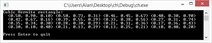
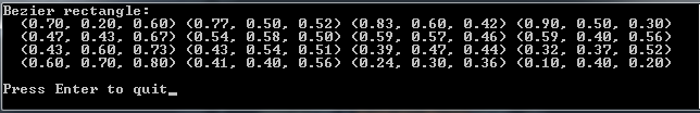
Here is the output of a run of the program:

What if I Need Constants?!

If you are thinking how you might actually use this code in a real setting, you might be thinking to yourself “it’s great to be able to multiply two encrypted numbers together, but what if I just need to multiply them by a constant like 43?”

Well, interestingly, you can literally just use 0 and 1 in this scheme as constants to perform operations against the encrypted bits.

The reason that this works is that you can see 0 and 1 as just very poor encryptions 😛

(0 % KEY) % 2 = 0
(1 % KEY) % 2 = 1

As long as KEY is >= 2, the above is always true, no matter what the key actually is!

So there you go, add your own constants into the calculations all you want. They also happen to have very low residue/error (actually, they have the least amount possible!), so are much more friendly to use, versus having someone provide you with an encrypted table of constants to use in your calculations. It’s also more secure for the person doing the encrypting for them to provide you less encrypted data that you know the plain text for. It limits your (and anyone else’s) ability to do a known plain text attack.

The Other Shoe Drops

You might notice that in our scheme, given the same key, every true bit will be the same value, and every false bit will be the same value. Unfortunately, the true bit is also always the false bit + 1. As an attacker, this means that once you have seen both a true bit and a false bit, you will then have broken the encryption.

Even worse, when you encrypt a false bit, it gives you back the key itself!

We’ll improve that in the next post by adding a few more simple operations to the encryption process.

This leveled HE encryption scheme comes directly from the paper below. If you want to give it a look, what we covered is only part of the first two pages!
Fully Homomorphic Encryption over the Integers

The links below are where I started reading up on HE. They go a different route with FHE that you might find interesting, and also have a lot more commentary about the usage cases of HE:
The Swiss Army Knife of Cryptography
Building the Swiss Army Knife

In the scheme in those links, I haven’t figured out how multiplication is supposed to work yet (or bootstrapping, but one thing at a time). If you figure it out, let me know!

Gaussian Blur

A web demo implements the formulas from this post at http://demofox.org/gauss.html

There is also this utility which has some real sophisticated features: https://github.com/manuelbua/blur-ninja

In this post we are going to take the concepts we went over in the last post (Box Blur) and apply them to Gaussian blurring.

At a high level, Gaussian blurring works just like box blurring in that there is a weight per pixel and that for each pixel, you apply the weights to that pixel and it’s neighbors to come up with the final value for the blurred pixel.

With true Gaussian blurring however, the function that defines the weights for each pixel technically never reaches zero, but gets smaller and smaller over distance. In theory this makes a Gaussian kernel infinitely large. In practice though, you can choose a cut off point and call it good enough.

The parameters to a Gaussian blur are:

  • Sigma (\sigma
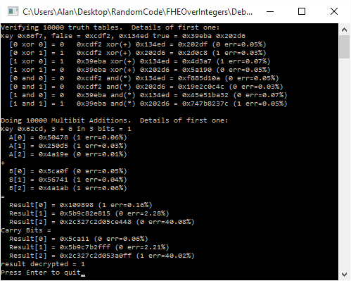
) – This defines how much blur there is. A larger number is a higher amount of blur.
  • Radius – The size of the kernel in pixels. The appropriate pixel size can be calculated for a specific sigma, but more information on that lower down.

Just like a box blur, a Gaussian blur is separable which means that you can either apply a 2d convolution kernel, or you can apply a 1d convolution kernel on each axis. Doing a single 2d convolution means more calculations, but you only need one buffer to put the results into. Doing two 1d convolutions (one on each axis), ends up being fewer calculations, but requires two buffers to put the results into (one intermediate buffer to hold the first axis results).

Here is a 3 pixel 1d Gaussian Kernel for a sigma of 1.0:

Below is a 3×3 pixel 2d Gaussian Kernel also with a sigma of 1.0. Note that this can be calculated as an outer product (tensor product) of 1d kernels!

An interesting property of Gaussian blurs is that you can apply multiple smaller blurs and it will come up with the result as if you did a larger Blur. Unfortunately it’s more calculations doing multiple smaller blurs so is not usually worth while.

If you apply multiple blurs, the equivalent blur is the square root of the sum of the squares of the blur. Taking wikipedia’s example, if you applied a blur with radius 6 and a blur with a radius of 8, you’d end up with the equivelant of a radius 10 blur. This is because \sqrt{6^2 + 8^2} = 10.

Calculating The Kernel

There are a couple ways to calculate a Gaussian kernel.

Believe it or not, Pascal’s triangle approaches the Gaussian bell curve as the row number reaches infinity. If you remember, Pascal’s triangle also represents the numbers that each term is calculated by after expanding binomials (x+y)^N. So technically, you could use a row from Pascal’s triangle as a 1d kernel and normalize the result, but it isn’t the most accurate.

A better way is to use the Gaussian function which is this:

e^{-x^2/(2*\sigma^2)}

Where the sigma is your blur amount and x ranges across your values from the negative to the positive. For instance if your kernel was 5 values, it would range from -2 to +2.

An even better way would be to integrate the Gaussian function instead of just taking point samples. You can read about it in the link at the bottom “Gaussian Kernel Calculator”, but it’s also what we do in the example code.

Whatever way you do it, make sure and normalize the result so that the weights add up to 1. This makes sure that your blurring doesn’t make the image get brighter (greater than 1) or dimmer (less than 1).

Calculating The Kernel Size

Given a sigma value, you can calculate the size of the kernel you need by using this formula:

1+2 \sqrt{-2 \sigma^2 \ln 0.005}

That formula makes a Kernel large enough such that it cuts off when the value in the kernel is less than 0.5%. You can adjust the number in there to higher or lower depending on your desires for speed versus quality.

Examples

Once again, here is the unaltered image we are working with:

Here is the image blurred with a sigma of 3,3 (3 on the x axis and 3 on the y axis):

Here is the image blurred with a sigma of 20,3:

Here is the image blurred with a sigma of 50,50:

Shadertoy

Here’s a shadertoy implementing Gaussian Blur: Shadertoy:DF Gaussian Blur

Code

Here’s the source code I used to blur the examples above:

#define _CRT_SECURE_NO_WARNINGS

#include &amp;lt;stdio.h&amp;gt;
#include &amp;lt;stdint.h&amp;gt;
#include &amp;lt;array&amp;gt;
#include &amp;lt;vector&amp;gt;
#include &amp;lt;functional&amp;gt;
#include &amp;lt;windows.h&amp;gt;  // for bitmap headers.  Sorry non windows people!

typedef uint8_t uint8;

const float c_pi = 3.14159265359f;

struct SImageData
{
    SImageData()
        : m_width(0)
        , m_height(0)
    { }

    long m_width;
    long m_height;
    long m_pitch;
    std::vector&amp;lt;uint8&amp;gt; m_pixels;
};

void WaitForEnter ()
{
    printf("Press Enter to quit");
    fflush(stdin);
    getchar();
}

bool LoadImage (const char *fileName, SImageData&amp;amp; imageData)
{
    // open the file if we can
    FILE *file;
    file = fopen(fileName, "rb");
    if (!file)
        return false;

    // read the headers if we can
    BITMAPFILEHEADER header;
    BITMAPINFOHEADER infoHeader;
    if (fread(&amp;amp;header, sizeof(header), 1, file) != 1 ||
        fread(&amp;amp;infoHeader, sizeof(infoHeader), 1, file) != 1 ||
        header.bfType != 0x4D42 || infoHeader.biBitCount != 24)
    {
        fclose(file);
        return false;
    }

    // read in our pixel data if we can. Note that it's in BGR order, and width is padded to the next power of 4
    imageData.m_pixels.resize(infoHeader.biSizeImage);
    fseek(file, header.bfOffBits, SEEK_SET);
    if (fread(&amp;amp;imageData.m_pixels[0], imageData.m_pixels.size(), 1, file) != 1)
    {
        fclose(file);
        return false;
    }

    imageData.m_width = infoHeader.biWidth;
    imageData.m_height = infoHeader.biHeight;

    imageData.m_pitch = imageData.m_width*3;
    if (imageData.m_pitch &amp;amp; 3)
    {
        imageData.m_pitch &amp;amp;= ~3;
        imageData.m_pitch += 4;
    }

    fclose(file);
    return true;
}

bool SaveImage (const char *fileName, const SImageData &amp;amp;image)
{
    // open the file if we can
    FILE *file;
    file = fopen(fileName, "wb");
    if (!file)
        return false;

    // make the header info
    BITMAPFILEHEADER header;
    BITMAPINFOHEADER infoHeader;

    header.bfType = 0x4D42;
    header.bfReserved1 = 0;
    header.bfReserved2 = 0;
    header.bfOffBits = 54;

    infoHeader.biSize = 40;
    infoHeader.biWidth = image.m_width;
    infoHeader.biHeight = image.m_height;
    infoHeader.biPlanes = 1;
    infoHeader.biBitCount = 24;
    infoHeader.biCompression = 0;
    infoHeader.biSizeImage = image.m_pixels.size();
    infoHeader.biXPelsPerMeter = 0;
    infoHeader.biYPelsPerMeter = 0;
    infoHeader.biClrUsed = 0;
    infoHeader.biClrImportant = 0;

    header.bfSize = infoHeader.biSizeImage + header.bfOffBits;

    // write the data and close the file
    fwrite(&amp;amp;header, sizeof(header), 1, file);
    fwrite(&amp;amp;infoHeader, sizeof(infoHeader), 1, file);
    fwrite(&amp;amp;image.m_pixels[0], infoHeader.biSizeImage, 1, file);
    fclose(file);
    return true;
}

int PixelsNeededForSigma (float sigma)
{
    // returns the number of pixels needed to represent a gaussian kernal that has values
    // down to the threshold amount.  A gaussian function technically has values everywhere
    // on the image, but the threshold lets us cut it off where the pixels contribute to
    // only small amounts that aren't as noticeable.
    const float c_threshold = 0.005f; // 0.5%
    return int(floor(1.0f + 2.0f * sqrtf(-2.0f * sigma * sigma * log(c_threshold)))) + 1;
}

float Gaussian (float sigma, float x)
{
    return expf(-(x*x) / (2.0f * sigma*sigma));
}

float GaussianSimpsonIntegration (float sigma, float a, float b)
{
    return
        ((b - a) / 6.0f) *
        (Gaussian(sigma, a) + 4.0f * Gaussian(sigma, (a + b) / 2.0f) + Gaussian(sigma, b));
}

std::vector&amp;lt;float&amp;gt; GaussianKernelIntegrals (float sigma, int taps)
{
    std::vector&amp;lt;float&amp;gt; ret;
    float total = 0.0f;
    for (int i = 0; i &amp;lt; taps; ++i)
    {
        float x = float(i) - float(taps / 2);
        float value = GaussianSimpsonIntegration(sigma, x - 0.5f, x + 0.5f);
        ret.push_back(value);
        total += value;
    }
    // normalize it
    for (unsigned int i = 0; i &amp;lt; ret.size(); ++i)
    {
        ret[i] /= total;
    }
    return ret;
}

const uint8* GetPixelOrBlack (const SImageData&amp;amp; image, int x, int y)
{
    static const uint8 black[3] = { 0, 0, 0 };
    if (x &amp;lt; 0 || x &amp;gt;= image.m_width ||
        y &amp;lt; 0 || y &amp;gt;= image.m_height)
    {
        return black;
    }

    return &amp;amp;image.m_pixels[(y * image.m_pitch) + x * 3];
}

void BlurImage (const SImageData&amp;amp; srcImage, SImageData &amp;amp;destImage, float xblursigma, float yblursigma, unsigned int xblursize, unsigned int yblursize)
{
    // allocate space for copying the image for destImage and tmpImage
    destImage.m_width = srcImage.m_width;
    destImage.m_height = srcImage.m_height;
    destImage.m_pitch = srcImage.m_pitch;
    destImage.m_pixels.resize(destImage.m_height * destImage.m_pitch);

    SImageData tmpImage;
    tmpImage.m_width = srcImage.m_width;
    tmpImage.m_height = srcImage.m_height;
    tmpImage.m_pitch = srcImage.m_pitch;
    tmpImage.m_pixels.resize(tmpImage.m_height * tmpImage.m_pitch);

    // horizontal blur from srcImage into tmpImage
    {
        auto row = GaussianKernelIntegrals(xblursigma, xblursize);

        int startOffset = -1 * int(row.size() / 2);

        for (int y = 0; y &amp;lt; tmpImage.m_height; ++y)
        {
            for (int x = 0; x &amp;lt; tmpImage.m_width; ++x)
            {
                std::array&amp;lt;float, 3&amp;gt; blurredPixel = { 0.0f, 0.0f, 0.0f };
                for (unsigned int i = 0; i &amp;lt; row.size(); ++i)
                {
                    const uint8 *pixel = GetPixelOrBlack(srcImage, x + startOffset + i, y);
                    blurredPixel[0] += float(pixel[0]) * row[i];
                    blurredPixel[1] += float(pixel[1]) * row[i];
                    blurredPixel[2] += float(pixel[2]) * row[i];
                }

                uint8 *destPixel = &amp;amp;tmpImage.m_pixels[y * tmpImage.m_pitch + x * 3];

                destPixel[0] = uint8(blurredPixel[0]);
                destPixel[1] = uint8(blurredPixel[1]);
                destPixel[2] = uint8(blurredPixel[2]);
            }
        }
    }

    // vertical blur from tmpImage into destImage
    {
        auto row = GaussianKernelIntegrals(yblursigma, yblursize);

        int startOffset = -1 * int(row.size() / 2);

        for (int y = 0; y &amp;lt; destImage.m_height; ++y)
        {
            for (int x = 0; x &amp;lt; destImage.m_width; ++x)
            {
                std::array&amp;lt;float, 3&amp;gt; blurredPixel = { 0.0f, 0.0f, 0.0f };
                for (unsigned int i = 0; i &amp;lt; row.size(); ++i)
                {
                    const uint8 *pixel = GetPixelOrBlack(tmpImage, x, y + startOffset + i);
                    blurredPixel[0] += float(pixel[0]) * row[i];
                    blurredPixel[1] += float(pixel[1]) * row[i];
                    blurredPixel[2] += float(pixel[2]) * row[i];
                }

                uint8 *destPixel = &amp;amp;destImage.m_pixels[y * destImage.m_pitch + x * 3];

                destPixel[0] = uint8(blurredPixel[0]);
                destPixel[1] = uint8(blurredPixel[1]);
                destPixel[2] = uint8(blurredPixel[2]);
            }
        }
    }
}

int main (int argc, char **argv)
{
    float xblursigma, yblursigma;

    bool showUsage = argc &amp;lt; 5 ||
        (sscanf(argv[3], "%f", &amp;amp;xblursigma) != 1) ||
        (sscanf(argv[4], "%f", &amp;amp;yblursigma) != 1);

    char *srcFileName = argv[1];
    char *destFileName = argv[2];

    if (showUsage)
    {
        printf("Usage: &amp;lt;source&amp;gt; &amp;lt;dest&amp;gt; &amp;lt;xblur&amp;gt; &amp;lt;yblur&amp;gt;nBlur values are sigmann");
        WaitForEnter();
        return 1;
    }

    // calculate pixel sizes, and make sure they are odd
    int xblursize = PixelsNeededForSigma(xblursigma) | 1;
    int yblursize = PixelsNeededForSigma(yblursigma) | 1;

    printf("Attempting to blur a 24 bit image.n");
    printf("  Source=%sn  Dest=%sn  blur=[%0.1f, %0.1f] px=[%d,%d]nn", srcFileName, destFileName, xblursigma, yblursigma, xblursize, yblursize);

    SImageData srcImage;
    if (LoadImage(srcFileName, srcImage))
    {
        printf("%s loadedn", srcFileName);
        SImageData destImage;
        BlurImage(srcImage, destImage, xblursigma, yblursigma, xblursize, yblursize);
        if (SaveImage(destFileName, destImage))
            printf("Blurred image saved as %sn", destFileName);
        else
        {
            printf("Could not save blurred image as %sn", destFileName);
            WaitForEnter();
            return 1;
        }
    }
    else
    {
        printf("could not read 24 bit bmp file %snn", srcFileName);
        WaitForEnter();
        return 1;
    }
    return 0;
}

Here is a really great explanation of the Gaussian blur.
Gaussian Blur – Image processing for scientists and engineers, Part 4
I highly recommend reading the 6 part series about image processing (DSP) from the beginning because it’s really informative and very easy to read!
Images are data – Image processing for scientists and engineers, Part 1

The Gaussian Kernel
Gaussian Kernel Calculator
DSP Stack Exchange: Gaussian Blur – standard deviation, radius and kernel size
Wikipedia: Gaussian blur

If you want to take this from theory / hobby level up to pro level, give this link a read from intel:
Intel: An investigation of fast real-time GPU-based image blur algorithms

Box Blur

If you ever have heard the terms “Box Blur”, “Boxcar Function”, “Box Filter”, “Boxcar Integrator” or other various combinations of those words, you may have thought it was some advanced concept that is hard to understand and hard to implement. If that’s what you thought, prepare to be surprised!

A box filter is nothing more than taking N samples of data (or NxN samples of data, or NxNxN etc) and averaging them! Yes, that is all there is to it 😛

In this post, we are going to implement a box blur by averaging pixels.

1D Case

For the case of a 1d box filter, let’s say we wanted every data point to be the result of averaging it with it’s two neighbors. It’d be easy enough to program that by just doing it, but let’s look at it a different way. What weight would we need to multiply each of the three values by (the value and it’s two neighbors) to make it come up with the average?

Yep, you guessed it! For every data value, you multiply it and it’s neighbors by 1/3 to come up with the average value. We could easily increase the size of the filter to 5 pixels, and multiply each pixel by 1/5 instead. We could continue the pattern as high as we wanted.

One thing you might notice is that if we want a buffer with all the results, we can’t just alter the source data as we go, because we want the unaltered source values of the data to use those weights with, to get the correct results. Because of that, we need to make a second buffer to put the results of the filtering into.

Believe it or not, that diagram above is a convolution kernel, and how we talked about applying it is how you do convolution in 1d! It just so happens that this convolution kernel averages three pixels into one, which also happens to provide a low pass filter type effect.

Low pass filtering is what is done before down sampling audio data to prevent aliasing (frequencies higher than the sample rate can handle, which makes audio sound bad).

Surprise… blurring can also be seen as low pass filtering, which is something you can do before scaling an image down in size, to prevent aliasing.

2D Case

The 2d case isn’t much more difficult to understand than the 1d case. Instead of only averaging on one axis, we average on two instead:

Something interesting to note is that you can either use this 3×3 2d convolution kernel, or, you could apply the 1d convolution kernel described above on the X axis and then the Y axis. The methods are mathematically equivalent.

Using the 2d convolution kernel would result in 9 multiplications per pixel, but if going with the separated axis X and then Y 1d kernel, you’d only end up doing 6 multiplications per pixel (3 multiplications per axis). In general, if you have a seperable 2d convolution kernel (meaning that you can break it into a per axis 1d convolution), you will end up doing N^2 multiplications when using the 2d kernel, versus N*2 multiplications when using the 1d kernels. You can see that this would add up quickly in favor of using 1d kernels, but unfortunately not all kernels are separable.

Doing two passes does come at a cost though. Since you have to use a temporary buffer for each pass, you end up having to create two temporary buffers instead of one.

You can build 2d kernels from 1d kernels by multiplying them as a row vector, by a column vector. For instance, you can see how multiplying the (1/3,1/3,1/3) kernel by itself as a column vector would create the 2nd kernel, that is 3×3 and has 1/9 in every spot.

The resulting 3×3 matrix is called an outer product, or a tensor product. Something interesting to note is that you don’t have to do the same operation on each axis!

Examples

Here are some examples of box blurring with different values, using the sample code provided below.

The source image:

Now blurred by a 10×10 box car convolution kernel:

Now blurred by a 100×10 box car convolution kernel:

Shadertoy

You can find a shadertoy implementation of box blurring here: Shadertoy:DF Box Blur

Code

Here’s the code I used to blur the example images above:

#define _CRT_SECURE_NO_WARNINGS
  
#include <stdio.h>
#include <stdint.h>
#include <array>
#include <vector>
#include <functional>
#include <windows.h>  // for bitmap headers.  Sorry non windows people!
  
typedef uint8_t uint8;
 
const float c_pi = 3.14159265359f;
 
struct SImageData
{
    SImageData()
        : m_width(0)
        , m_height(0)
    { }
  
    long m_width;
    long m_height;
    long m_pitch;
    std::vector<uint8> m_pixels;
};
  
void WaitForEnter ()
{
    printf("Press Enter to quit");
    fflush(stdin);
    getchar();
}
  
bool LoadImage (const char *fileName, SImageData& imageData)
{
    // open the file if we can
    FILE *file;
    file = fopen(fileName, "rb");
    if (!file)
        return false;
  
    // read the headers if we can
    BITMAPFILEHEADER header;
    BITMAPINFOHEADER infoHeader;
    if (fread(&header, sizeof(header), 1, file) != 1 ||
        fread(&infoHeader, sizeof(infoHeader), 1, file) != 1 ||
        header.bfType != 0x4D42 || infoHeader.biBitCount != 24)
    {
        fclose(file);
        return false;
    }
  
    // read in our pixel data if we can. Note that it's in BGR order, and width is padded to the next power of 4
    imageData.m_pixels.resize(infoHeader.biSizeImage);
    fseek(file, header.bfOffBits, SEEK_SET);
    if (fread(&imageData.m_pixels[0], imageData.m_pixels.size(), 1, file) != 1)
    {
        fclose(file);
        return false;
    }
  
    imageData.m_width = infoHeader.biWidth;
    imageData.m_height = infoHeader.biHeight;
  
    imageData.m_pitch = imageData.m_width*3;
    if (imageData.m_pitch & 3)
    {
        imageData.m_pitch &= ~3;
        imageData.m_pitch += 4;
    }
  
    fclose(file);
    return true;
}
  
bool SaveImage (const char *fileName, const SImageData &image)
{
    // open the file if we can
    FILE *file;
    file = fopen(fileName, "wb");
    if (!file)
        return false;
  
    // make the header info
    BITMAPFILEHEADER header;
    BITMAPINFOHEADER infoHeader;
  
    header.bfType = 0x4D42;
    header.bfReserved1 = 0;
    header.bfReserved2 = 0;
    header.bfOffBits = 54;
  
    infoHeader.biSize = 40;
    infoHeader.biWidth = image.m_width;
    infoHeader.biHeight = image.m_height;
    infoHeader.biPlanes = 1;
    infoHeader.biBitCount = 24;
    infoHeader.biCompression = 0;
    infoHeader.biSizeImage = image.m_pixels.size();
    infoHeader.biXPelsPerMeter = 0;
    infoHeader.biYPelsPerMeter = 0;
    infoHeader.biClrUsed = 0;
    infoHeader.biClrImportant = 0;
  
    header.bfSize = infoHeader.biSizeImage + header.bfOffBits;
  
    // write the data and close the file
    fwrite(&header, sizeof(header), 1, file);
    fwrite(&infoHeader, sizeof(infoHeader), 1, file);
    fwrite(&image.m_pixels[0], infoHeader.biSizeImage, 1, file);
    fclose(file);
    return true;
}

const uint8* GetPixelOrBlack (const SImageData& image, int x, int y)
{
    static const uint8 black[3] = { 0, 0, 0 };
    if (x < 0 || x >= image.m_width ||
        y < 0 || y >= image.m_height)
    {
        return black;
    }
 
    return &image.m_pixels[(y * image.m_pitch) + x * 3];
}
 
void BlurImage (const SImageData& srcImage, SImageData &destImage, unsigned int xblur, unsigned int yblur)
{
    // allocate space for copying the image for destImage and tmpImage
    destImage.m_width = srcImage.m_width;
    destImage.m_height = srcImage.m_height;
    destImage.m_pitch = srcImage.m_pitch;
    destImage.m_pixels.resize(destImage.m_height * destImage.m_pitch);
 
    SImageData tmpImage;
    tmpImage.m_width = srcImage.m_width;
    tmpImage.m_height = srcImage.m_height;
    tmpImage.m_pitch = srcImage.m_pitch;
    tmpImage.m_pixels.resize(tmpImage.m_height * tmpImage.m_pitch);
 
    // horizontal blur from srcImage into tmpImage
    {
        float weight = 1.0f / float(xblur);
        int half = xblur / 2;
        for (int y = 0; y < tmpImage.m_height; ++y)
        {
            for (int x = 0; x < tmpImage.m_width; ++x)
            {
                std::array<float, 3> blurredPixel = { 0.0f, 0.0f, 0.0f };
                for (int i = -half; i <= half; ++i)
                {
                    const uint8 *pixel = GetPixelOrBlack(srcImage, x + i, y);
                    blurredPixel[0] += float(pixel[0]) * weight;
                    blurredPixel[1] += float(pixel[1]) * weight;
                    blurredPixel[2] += float(pixel[2]) * weight;
                }
                 
                uint8 *destPixel = &tmpImage.m_pixels[y * tmpImage.m_pitch + x * 3];
 
                destPixel[0] = uint8(blurredPixel[0]);
                destPixel[1] = uint8(blurredPixel[1]);
                destPixel[2] = uint8(blurredPixel[2]);
            }
        }
    }
 
    // vertical blur from tmpImage into destImage
    {
        float weight = 1.0f / float(yblur);
        int half = yblur / 2;
 
        for (int y = 0; y < destImage.m_height; ++y)
        {
            for (int x = 0; x < destImage.m_width; ++x)
            {
                std::array<float, 3> blurredPixel = { 0.0f, 0.0f, 0.0f };
                for (int i = -half; i <= half; ++i)
                {
                    const uint8 *pixel = GetPixelOrBlack(tmpImage, x, y + i);
                    blurredPixel[0] += float(pixel[0]) * weight;
                    blurredPixel[1] += float(pixel[1]) * weight;
                    blurredPixel[2] += float(pixel[2]) * weight;
                }
 
                uint8 *destPixel = &destImage.m_pixels[y * destImage.m_pitch + x * 3];
 
                destPixel[0] = uint8(blurredPixel[0]);
                destPixel[1] = uint8(blurredPixel[1]);
                destPixel[2] = uint8(blurredPixel[2]);
            }
        }
    }
}
 
int main (int argc, char **argv)
{
    int xblur, yblur;
  
    bool showUsage = argc < 5 ||
        (sscanf(argv[3], "%i", &xblur) != 1) ||
        (sscanf(argv[4], "%i", &yblur) != 1);
  
    char *srcFileName = argv[1];
    char *destFileName = argv[2];
  
    if (showUsage)
    {
        printf("Usage: <source> <dest> <xblur> <yblur>nn");
        WaitForEnter();
        return 1;
    }
     
    // make sure blur size is odd
    xblur = xblur | 1;
    yblur = yblur | 1;
 
    printf("Attempting to blur a 24 bit image.n");
    printf("  Source=%sn  Dest=%sn  blur=[%d,%d]nn", srcFileName, destFileName, xblur, yblur);
  
    SImageData srcImage;
    if (LoadImage(srcFileName, srcImage))
    {
        printf("%s loadedn", srcFileName);
        SImageData destImage;
        BlurImage(srcImage, destImage, xblur, yblur);
        if (SaveImage(destFileName, destImage))
            printf("Blurred image saved as %sn", destFileName);
        else
        {
            printf("Could not save blurred image as %sn", destFileName);
            WaitForEnter();
            return 1;
        }
    }
    else
    {
        printf("could not read 24 bit bmp file %snn", srcFileName);
        WaitForEnter();
        return 1;
    }
    return 0;
}

Next Up

Next up will be a Gaussian blur, and I’m nearly done w/ that post but wanted to make this one first as an introductory step!

Before we get there, I wanted to mention that if you do multiple box blurs in a row, it will start to approach Gaussian blurring. I’ve heard that three blurs in a row will make it basically indistinguishable from a Gaussian blur.

Resizing Images With Bicubic Interpolation

In the last post we saw how to do cubic interpolation on a grid of data.

Strangely enough, when that grid is a grid of pixel data, bicubic interpolation is a common method for resizing images!

Bicubic interpolation can also used in realtime rendering to make textures look nicer when scaled than standard bilinear texture interpolation.

This technique works when making images larger as well as smaller, but when making images smaller, you can still have problems with aliasing. There are are better algorithms to use when making an image smaller. Check the links section at the bottom for more details!

Example

Here’s the old man from The Legend of Zelda who gives you the sword.

Here he is scaled up 4x with nearest neighbor, bilinear interpolation and bicubic interpolation.


Here he is scaled up 16x with nearest neighbor, bilinear interpolation and bicubic interpolation.


Shadertoy

I made a shadertoy to show you how to do this in a GLSL pixel shader as well. Shadertoy: Bicubic Texture Filtering

In the screenshot below, going from left to right it uses: Nearest Neighbor, Bilinear, Lagrange Bicubic interpolation (only interpolates values, not slopes), Hermite Bicubic interpolation.

Sample Code

Here’s the code that I used to resize the images in the examples above.

#define _CRT_SECURE_NO_WARNINGS

#include <stdio.h>
#include <stdint.h>
#include <array>
#include <vector>
#include <windows.h>  // for bitmap headers.  Sorry non windows people!

#define CLAMP(v, min, max) if (v < min) { v = min; } else if (v > max) { v = max; } 

typedef uint8_t uint8;

struct SImageData
{
    SImageData()
        : m_width(0)
        , m_height(0)
    { }

    long m_width;
    long m_height;
    long m_pitch;
    std::vector<uint8> m_pixels;
};

void WaitForEnter ()
{
    printf("Press Enter to quit");
    fflush(stdin);
    getchar();
}

bool LoadImage (const char *fileName, SImageData& imageData)
{
    // open the file if we can
    FILE *file;
    file = fopen(fileName, "rb");
    if (!file)
        return false;

    // read the headers if we can
    BITMAPFILEHEADER header;
    BITMAPINFOHEADER infoHeader;
    if (fread(&header, sizeof(header), 1, file) != 1 ||
        fread(&infoHeader, sizeof(infoHeader), 1, file) != 1 ||
        header.bfType != 0x4D42 || infoHeader.biBitCount != 24)
    {
        fclose(file);
        return false;
    }

    // read in our pixel data if we can. Note that it's in BGR order, and width is padded to the next power of 4
    imageData.m_pixels.resize(infoHeader.biSizeImage);
    fseek(file, header.bfOffBits, SEEK_SET);
    if (fread(&imageData.m_pixels[0], imageData.m_pixels.size(), 1, file) != 1)
    {
        fclose(file);
        return false;
    }

    imageData.m_width = infoHeader.biWidth;
    imageData.m_height = infoHeader.biHeight;

    imageData.m_pitch = imageData.m_width*3;
    if (imageData.m_pitch & 3)
    {
        imageData.m_pitch &= ~3;
        imageData.m_pitch += 4;
    }

    fclose(file);
    return true;
}

bool SaveImage (const char *fileName, const SImageData &image)
{
    // open the file if we can
    FILE *file;
    file = fopen(fileName, "wb");
    if (!file)
        return false;

    // make the header info
    BITMAPFILEHEADER header;
    BITMAPINFOHEADER infoHeader;

    header.bfType = 0x4D42;
    header.bfReserved1 = 0;
    header.bfReserved2 = 0;
    header.bfOffBits = 54;

    infoHeader.biSize = 40;
    infoHeader.biWidth = image.m_width;
    infoHeader.biHeight = image.m_height;
    infoHeader.biPlanes = 1;
    infoHeader.biBitCount = 24;
    infoHeader.biCompression = 0;
    infoHeader.biSizeImage = image.m_pixels.size();
    infoHeader.biXPelsPerMeter = 0;
    infoHeader.biYPelsPerMeter = 0;
    infoHeader.biClrUsed = 0;
    infoHeader.biClrImportant = 0;

    header.bfSize = infoHeader.biSizeImage + header.bfOffBits;

    // write the data and close the file
    fwrite(&header, sizeof(header), 1, file);
    fwrite(&infoHeader, sizeof(infoHeader), 1, file);
    fwrite(&image.m_pixels[0], infoHeader.biSizeImage, 1, file);
    fclose(file);
    return true;
}

// t is a value that goes from 0 to 1 to interpolate in a C1 continuous way across uniformly sampled data points.
// when t is 0, this will return B.  When t is 1, this will return C.  Inbetween values will return an interpolation
// between B and C.  A and B are used to calculate slopes at the edges.
float CubicHermite (float A, float B, float C, float D, float t)
{
    float a = -A / 2.0f + (3.0f*B) / 2.0f - (3.0f*C) / 2.0f + D / 2.0f;
    float b = A - (5.0f*B) / 2.0f + 2.0f*C - D / 2.0f;
    float c = -A / 2.0f + C / 2.0f;
    float d = B;

    return a*t*t*t + b*t*t + c*t + d;
}

float Lerp (float A, float B, float t)
{
    return A * (1.0f - t) + B * t;
}

const uint8* GetPixelClamped (const SImageData& image, int x, int y)
{
    CLAMP(x, 0, image.m_width - 1);
    CLAMP(y, 0, image.m_height - 1);    
    return &image.m_pixels[(y * image.m_pitch) + x * 3];
}

std::array<uint8, 3> SampleNearest (const SImageData& image, float u, float v)
{
    // calculate coordinates
    int xint = int(u * image.m_width);
    int yint = int(v * image.m_height);

    // return pixel
    auto pixel = GetPixelClamped(image, xint, yint);
    std::array<uint8, 3> ret;
    ret[0] = pixel[0];
    ret[1] = pixel[1];
    ret[2] = pixel[2];
    return ret;
}

std::array<uint8, 3> SampleLinear (const SImageData& image, float u, float v)
{
    // calculate coordinates -> also need to offset by half a pixel to keep image from shifting down and left half a pixel
    float x = (u * image.m_width) - 0.5f;
    int xint = int(x);
    float xfract = x - floor(x);

    float y = (v * image.m_height) - 0.5f;
    int yint = int(y);
    float yfract = y - floor(y);

    // get pixels
    auto p00 = GetPixelClamped(image, xint + 0, yint + 0);
    auto p10 = GetPixelClamped(image, xint + 1, yint + 0);
    auto p01 = GetPixelClamped(image, xint + 0, yint + 1);
    auto p11 = GetPixelClamped(image, xint + 1, yint + 1);

    // interpolate bi-linearly!
    std::array<uint8, 3> ret;
    for (int i = 0; i < 3; ++i)
    {
        float col0 = Lerp(p00[i], p10[i], xfract);
        float col1 = Lerp(p01[i], p11[i], xfract);
        float value = Lerp(col0, col1, yfract);
        CLAMP(value, 0.0f, 255.0f);
        ret[i] = uint8(value);
    }
    return ret;
}

std::array<uint8, 3> SampleBicubic (const SImageData& image, float u, float v)
{
    // calculate coordinates -> also need to offset by half a pixel to keep image from shifting down and left half a pixel
    float x = (u * image.m_width) - 0.5;
    int xint = int(x);
    float xfract = x - floor(x);

    float y = (v * image.m_height) - 0.5;
    int yint = int(y);
    float yfract = y - floor(y);

    // 1st row
    auto p00 = GetPixelClamped(image, xint - 1, yint - 1);
    auto p10 = GetPixelClamped(image, xint + 0, yint - 1);
    auto p20 = GetPixelClamped(image, xint + 1, yint - 1);
    auto p30 = GetPixelClamped(image, xint + 2, yint - 1);

    // 2nd row
    auto p01 = GetPixelClamped(image, xint - 1, yint + 0);
    auto p11 = GetPixelClamped(image, xint + 0, yint + 0);
    auto p21 = GetPixelClamped(image, xint + 1, yint + 0);
    auto p31 = GetPixelClamped(image, xint + 2, yint + 0);

    // 3rd row
    auto p02 = GetPixelClamped(image, xint - 1, yint + 1);
    auto p12 = GetPixelClamped(image, xint + 0, yint + 1);
    auto p22 = GetPixelClamped(image, xint + 1, yint + 1);
    auto p32 = GetPixelClamped(image, xint + 2, yint + 1);

    // 4th row
    auto p03 = GetPixelClamped(image, xint - 1, yint + 2);
    auto p13 = GetPixelClamped(image, xint + 0, yint + 2);
    auto p23 = GetPixelClamped(image, xint + 1, yint + 2);
    auto p33 = GetPixelClamped(image, xint + 2, yint + 2);

    // interpolate bi-cubically!
    // Clamp the values since the curve can put the value below 0 or above 255
    std::array<uint8, 3> ret;
    for (int i = 0; i < 3; ++i)
    {
        float col0 = CubicHermite(p00[i], p10[i], p20[i], p30[i], xfract);
        float col1 = CubicHermite(p01[i], p11[i], p21[i], p31[i], xfract);
        float col2 = CubicHermite(p02[i], p12[i], p22[i], p32[i], xfract);
        float col3 = CubicHermite(p03[i], p13[i], p23[i], p33[i], xfract);
        float value = CubicHermite(col0, col1, col2, col3, yfract);
        CLAMP(value, 0.0f, 255.0f);
        ret[i] = uint8(value);
    }
    return ret;
}

void ResizeImage (const SImageData &srcImage, SImageData &destImage, float scale, int degree)
{
    destImage.m_width = long(float(srcImage.m_width)*scale);
    destImage.m_height = long(float(srcImage.m_height)*scale);
    destImage.m_pitch = destImage.m_width * 3;
    if (destImage.m_pitch & 3)
    {
        destImage.m_pitch &= ~3;
        destImage.m_pitch += 4;
    }
    destImage.m_pixels.resize(destImage.m_pitch*destImage.m_height);

    uint8 *row = &destImage.m_pixels[0];
    for (int y = 0; y < destImage.m_height; ++y)
    {
        uint8 *destPixel = row;
        float v = float(y) / float(destImage.m_height - 1);
        for (int x = 0; x < destImage.m_width; ++x)
        {
            float u = float(x) / float(destImage.m_width - 1);
            std::array<uint8, 3> sample;

            if (degree == 0)
                sample = SampleNearest(srcImage, u, v);
            else if (degree == 1)
                sample = SampleLinear(srcImage, u, v);
            else if (degree == 2)
                sample = SampleBicubic(srcImage, u, v);

            destPixel[0] = sample[0];
            destPixel[1] = sample[1];
            destPixel[2] = sample[2];
            destPixel += 3;
        }
        row += destImage.m_pitch;
    }
}

int main (int argc, char **argv)
{
    float scale = 1.0f;
    int degree = 0;

    bool showUsage = argc < 5 ||
        (sscanf(argv[3], "%f", &scale) != 1) ||
        (sscanf(argv[4], "%i", &degree) != 1);

    char *srcFileName = argv[1];
    char *destFileName = argv[2];

    if (showUsage)
    {
        printf("Usage: <source> <dest> <scale> <degree>ndegree 0 = nearest, 1 = bilinear, 2 = bicubic.nn");
        WaitForEnter();
        return 1;
    }

    printf("Attempting to resize a 24 bit image.n");
    printf("  Source = %sn  Dest = %sn  Scale = %0.2fnn", srcFileName, destFileName, scale);

    SImageData srcImage;
    if (LoadImage(srcFileName, srcImage))
    {
        printf("%s loadedn", srcFileName);
        SImageData destImage;
        ResizeImage(srcImage, destImage, scale, degree);
        if (SaveImage(destFileName, destImage))
            printf("Resized image saved as %sn", destFileName);
        else
            printf("Could not save resized image as %sn", destFileName);
    }
    else
        printf("could not read 24 bit bmp file %snn", srcFileName);
    return 0;
}

Links

A small tutorial about how to load a bitmap file
The BMP Format
Reconstruction Filters in Computer Graphics

The link below talks about how to do cubic texture sampling on the GPU without having to do 16 texture reads!
GPU Gems 2 Chapter 20. Fast Third-Order Texture Filtering

This link is from Inigo Quilez, where he transforms a texture coordinate before passing it to the bilinear filtering, to get higher quality texture sampling without having to do extra texture reads. That is pretty cool.
IQ: improved texture interpolation

Cubic Hermite Rectangles

Time for another Frankenstein post. This time we are going to combine the following:

  1. Cubic Hermite Interpolation
  2. Rectangular Bezier Patches

The end result is going to be a Cubic Hermite Rectangle Surface like the below. Note that the curve only passes through the inner four control points, and the outer ring of 12 control points are used to determine the slope.

Just like the cubic hermite curve counterpart, a cubic hermite rectangle surface is C1 continuous everywhere, which is great for use as a way of modeling geometry, as well as just for interpolation of multidimensional data. In the image below, each checkerboard square is an individual hermite rectangle.

The links section at the bottom has links to the shadertoys I made that I got the screenshots from.

Code

Here’s some C++ code that does bicubic hermite interpolation

#include <stdio.h>
#include <array>
  
typedef std::array<float, 4> TFloat4;
typedef std::array<TFloat4, 4> TFloat4x4;
  
const TFloat4x4 c_ControlPointsX =
{
    {
        { 0.7f, 0.8f, 0.9f, 0.3f },
        { 0.2f, 0.5f, 0.4f, 0.1f },
        { 0.6f, 0.3f, 0.1f, 0.4f },
        { 0.8f, 0.4f, 0.2f, 0.7f },
    }
};
  
const TFloat4x4 c_ControlPointsY =
{
    {
        { 0.2f, 0.8f, 0.5f, 0.6f },
        { 0.6f, 0.9f, 0.3f, 0.8f },
        { 0.7f, 0.1f, 0.4f, 0.9f },
        { 0.6f, 0.5f, 0.3f, 0.2f },
    }
};
  
const TFloat4x4 c_ControlPointsZ =
{
    {
        { 0.6f, 0.5f, 0.3f, 0.2f },
        { 0.7f, 0.1f, 0.9f, 0.5f },
        { 0.8f, 0.4f, 0.2f, 0.7f },
        { 0.6f, 0.3f, 0.1f, 0.4f },
    }
};
  
void WaitForEnter ()
{
    printf("Press Enter to quit");
    fflush(stdin);
    getchar();
}
  
// t is a value that goes from 0 to 1 to interpolate in a C1 continuous way across uniformly sampled data points.
// when t is 0, this will return p[1].  When t is 1, this will return p[2].
// p[0] and p[3] are used to calculate slopes at the edges.
float CubicHermite(const TFloat4& p, float t)
{
    float a = -p[0] / 2.0f + (3.0f*p[1]) / 2.0f - (3.0f*p[2]) / 2.0f + p[3] / 2.0f;
    float b = p[0] - (5.0f*p[1]) / 2.0f + 2.0f*p[2] - p[3] / 2.0f;
    float c = -p[0] / 2.0f + p[2] / 2.0f;
    float d = p[1];

    return a*t*t*t + b*t*t + c*t + d;
}
  
float BicubicHermitePatch(const TFloat4x4& p, float u, float v)
{
    TFloat4 uValues;
    uValues[0] = CubicHermite(p[0], u);
    uValues[1] = CubicHermite(p[1], u);
    uValues[2] = CubicHermite(p[2], u);
    uValues[3] = CubicHermite(p[2], u);
    return CubicHermite(uValues, v);
}
  
int main(int argc, char **argv)
{
    // how many values to display on each axis. Limited by console resolution!
    const int c_numValues = 4;
  
    printf("Cubic Hermite rectangle:n");
    for (int i = 0; i < c_numValues; ++i)
    {
        float iPercent = ((float)i) / ((float)(c_numValues - 1));
        for (int j = 0; j < c_numValues; ++j)
        {
            if (j == 0)
                printf("  ");
            float jPercent = ((float)j) / ((float)(c_numValues - 1));
            float valueX = BicubicHermitePatch(c_ControlPointsX, jPercent, iPercent);
            float valueY = BicubicHermitePatch(c_ControlPointsY, jPercent, iPercent);
            float valueZ = BicubicHermitePatch(c_ControlPointsZ, jPercent, iPercent);
            printf("(%0.2f, %0.2f, %0.2f) ", valueX, valueY, valueZ);
        }
        printf("n");
    }
    printf("n");
  
    WaitForEnter();
    return 0;
}

And here’s the output. Note that the four corners of the output correspond to the four inner most points defined in the data!

On The GPU / Links

While cubic Hermite rectangles pass through all of their control points like Lagrange surfaces do (and like Bezier rectangle’s don’t), they don’t suffer from Runge’s Phenomenon like Lagrange surfaces do.

However, just like Lagrange surfaces, Hermite surfaces don’t have the nice property that Bezier surfaces have, where the surface is guaranteed to stay inside of the convex hull defined by the control points.

Since Hermite surfaces are just cubic functions though, you could calculate the minimum and maximum value that they can reach using some calculus and come up with a bounding box by going that direction. The same thing is technically true of Lagrange surfaces as well for what it’s worth.

Check out the links below to see cubic Hermite rectangles rendered in real time in WebGL using raytracing and raymarching:
Shadertoy: Cubic Hermite Rectangle
Shadertoy: Infinite Hermite Rectangles

Cubic Hermite Interpolation

It’s a big wide world of curves out there and I have to say that most of the time, I consider myself a Bezier man.

Well let me tell you… cubic Hermite splines are technically representable in Bezier form, but they have some really awesome properties that I never fully appreciated until recently.

Usefulness For Interpolation

If you have a set of data points on some fixed interval (like for audio data, but could be anything), you can use a cubic Hermite spline to interpolate between any two data points. It interpolates the value between those points (as in, it passes through both end points), but it also interpolates a derivative that is consistent if you approach the point from the left or the right.

In short, this means you can use cubic Hermite splines to interpolate data such that the result has C1 continuity everywhere!

Usefulness As Curves

If you have any number N control points on a fixed interval, you can treat it as a bunch of piece wise cubic Hermite splines and evaluate it that way.

The end result is that you have a curve that is C1 continuous everywhere, it has local control (moving any control point only affects the two curve sections to the left and the two curve sections to the right), and best of all, the computational complexity doesn’t rise as you increase the number of control points!

The image below was taken as a screenshot from one of the HTML5 demos I made for you to play with. You can find links to them at the end of this post.

Cubic Hermite Splines

Cubic Hermite splines have four control points but how it uses the control points is a bit different than you’d expect.

The curve itself passes only through the middle two control points, and the end control points are there to help calculate the tangent at the middle control points.

Let’s say you have control points P_{-1}, P_0, P_1, P_2. The curve at time 0 will be at point P_0 and the slope will be the same slope as a line would have if going from P_{-1} to P_1. The curve at time 1 will be at point P_1 and the slope will be the same slope as a line would have if going from P_0 to P_2.

Check out the picture below to see what I mean visually.

That sounds like a strange set of properties, but they are actually super useful.

What this means is that you can treat any group of 4 control points / data points as a separate cubic hermite spline, but when you put it all together, it is a single smooth curve.

Note that you can either interpolate 1d data, or you can interpolate 2d data points by doing this interpolation on each axis. You could also use this to make a surface, which will likely be the next blog post!

The Math

I won’t go into how the formula is derived, but if you are interested you should check out Signal Processing: Bicubic Interpolation.

The formula is:

a*t^3+b*t^2+c*t+d

Where…

a = \frac{-P_{-1} + 3*P_0 - 3*P_1 + P_2}{2}
b = P_{-1} - \frac{5*P_0}{2} + 2*P_1 - \frac{P_2}{2}
c = \frac{-P_{-1} + P_1}{2}
d = P_0

Note that t is a value that goes from 0 to 1. When t is 0, your curve will be at P_1 and when t is 1, your curve will be at P_2. P_{-1} and P_{2} 
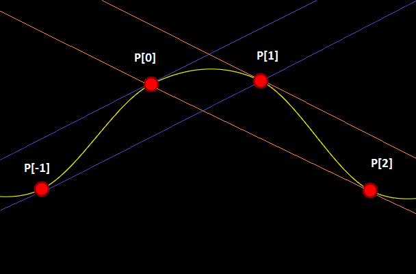
are used to be able to make this interpolation C1 continuous.

Here it is in some simple C++:

// t is a value that goes from 0 to 1 to interpolate in a C1 continuous way across uniformly sampled data points.
// when t is 0, this will return B.  When t is 1, this will return C.
static float CubicHermite (float A, float B, float C, float D, float t)
{
    float a = -A/2.0f + (3.0f*B)/2.0f - (3.0f*C)/2.0f + D/2.0f;
    float b = A - (5.0f*B)/2.0f + 2.0f*C - D / 2.0f;
    float c = -A/2.0f + C/2.0f;
    float d = B;

    return a*t*t*t + b*t*t + c*t + d;
}

Code

Here is an example C++ program that interpolates both 1D and 2D data.

#include <stdio.h>
#include <vector>
#include <array>
 
typedef std::vector<float> TPointList1D;
typedef std::vector<std::array<float,2>> TPointList2D;
 
void WaitForEnter ()
{
    printf("Press Enter to quit");
    fflush(stdin);
    getchar();
}

// t is a value that goes from 0 to 1 to interpolate in a C1 continuous way across uniformly sampled data points.
// when t is 0, this will return B.  When t is 1, this will return C.
float CubicHermite (float A, float B, float C, float D, float t)
{
    float a = -A/2.0f + (3.0f*B)/2.0f - (3.0f*C)/2.0f + D/2.0f;
    float b = A - (5.0f*B)/2.0f + 2.0f*C - D / 2.0f;
    float c = -A/2.0f + C/2.0f;
    float d = B;
 
    return a*t*t*t + b*t*t + c*t + d;
}

template <typename T>
inline T GetIndexClamped(const std::vector<T>& points, int index)
{
    if (index < 0)
        return points[0];
    else if (index >= int(points.size()))
        return points.back();
    else
        return points[index];
}

int main (int argc, char **argv)
{
    const float c_numSamples = 13;

    // show some 1d interpolated values
    {
        const TPointList1D points =
        {
            0.0f,
            1.6f,
            2.3f,
            3.5f,
            4.3f,
            5.9f,
            6.8f
        };

        printf("1d interpolated values.  y = f(t)n");
        for (int i = 0; i < c_numSamples; ++i)
        {
            float percent = ((float)i) / (float(c_numSamples - 1));
            float x = (points.size()-1) * percent;

            int index = int(x);
            float t = x - floor(x);
            float A = GetIndexClamped(points, index - 1);
            float B = GetIndexClamped(points, index + 0);
            float C = GetIndexClamped(points, index + 1);
            float D = GetIndexClamped(points, index + 2);

            float y = CubicHermite(A, B, C, D, t);
            printf("  Value at %0.2f = %0.2fn", x, y);
        }
        printf("n");
    }

    // show some 2d interpolated values
    {
        const TPointList2D points =
        {
            { 0.0f, 1.1f },
            { 1.6f, 8.3f },
            { 2.3f, 6.5f },
            { 3.5f, 4.7f },
            { 4.3f, 3.1f },
            { 5.9f, 7.5f },
            { 6.8f, 0.0f }
        };

        printf("2d interpolated values.  x = f(t), y = f(t)n");
        for (int i = 0; i < c_numSamples; ++i)
        {
            float percent = ((float)i) / (float(c_numSamples - 1));
            float x = 0.0f;
            float y = 0.0f;

            float tx = (points.size() -1) * percent;
            int index = int(tx);
            float t = tx - floor(tx);

            std::array<float, 2> A = GetIndexClamped(points, index - 1);
            std::array<float, 2> B = GetIndexClamped(points, index + 0);
            std::array<float, 2> C = GetIndexClamped(points, index + 1);
            std::array<float, 2> D = GetIndexClamped(points, index + 2);
            x = CubicHermite(A[0], B[0], C[0], D[0], t);
            y = CubicHermite(A[1], B[1], C[1], D[1], t);

            printf("  Value at %0.2f = (%0.2f, %0.2f)n", tx, x, y);
        }
        printf("n");
    }
 
    WaitForEnter();
    return 0;
}

The output of the program is below:

Links

Here are some interactive HTML5 demos i made:
1D cubic hermite interpolation
2D cubic hermite interpolation

More info here:
Wikipedia: Cubic Hermite Spline

Closely related to cubic hermite splines, catmull-rom splines allow you to specify a “tension” parameter to make the result more or less curvy:
Catmull-Rom spline

Lagrange Rectangles

In this post we are going to Frankenstein ideas from two other recent posts. If you haven’t seen these yet you should probably give them a read!

Ingredient 1: Lagrange interpolation
Ingredient 2: Rectangular Bezier Patches

Lagrange Surface

Lets say you have a grid of size MxN and you want to make a 3d surface for that grid.

You could use a Bezier rectangle but lets say that you really need the surface to pass through the control points. Bezier curves and surfaces only generally pass through the end / edge control points.

So what do you do? How about using Lagrange interpolation instead?

Just like how Bezier rectangles work, you interpolate on one axis, and then take those values and interpolate on the other axis.

Doing that, you get something like the below:

This comes at a price though. Whereas a Bezier curve or surface will be completely contained by it’s control points, a Lagrange rectangle isn’t always. Also, they are subject to something called Runge’s Phenomenon which basically means that the more control points you add, the more likely a surface is to get a bit “squirly”. You can see this effect when you add a lot of control points to my 1d lagrange interpolation demo as well: HTML5 1d Lagrange Interpolation.

Below is a picture of a bicubic Lagrange rectangle using the same control points the cubic Bezier rectangles used. Notice how much more extreme the peaks and valleys are! In the screenshot above, i scaled down the control points to 1/3 of what they were in the Bezier demo to make it look more reasonably well behaved.

Code

#include <stdio.h>
#include <array>
 
typedef std::array<float, 3> TFloat3;
typedef std::array<TFloat3, 3> TFloat3x3;
 
const TFloat3x3 c_ControlPointsX =
{
    {
        { 0.7f, 0.8f, 0.9f },
        { 0.2f, 0.5f, 0.4f },
        { 0.6f, 0.3f, 0.1f },
    }
};
 
const TFloat3x3 c_ControlPointsY =
{
    {
        { 0.2f, 0.8f, 0.5f },
        { 0.6f, 0.9f, 0.3f },
        { 0.7f, 0.1f, 0.4f },
    }
};
 
const TFloat3x3 c_ControlPointsZ =
{
    {
        { 0.6f, 0.5f, 0.3f },
        { 0.7f, 0.1f, 0.9f },
        { 0.8f, 0.4f, 0.2f },
    }
};
 
void WaitForEnter ()
{
    printf("Press Enter to quit");
    fflush(stdin);
    getchar();
}
 
//=======================================================================================
float QuadraticLagrange (const TFloat3& p, float t)
{
	float c_x0 = 0.0 / 2.0;
	float c_x1 = 1.0 / 2.0;
	float c_x2 = 2.0 / 2.0;

    return
        p[0] * 
        (
            (t - c_x1) / (c_x0 - c_x1) * 
            (t - c_x2) / (c_x0 - c_x2)
        ) +
        p[1] * 
        (
            (t - c_x0) / (c_x1 - c_x0) * 
            (t - c_x2) / (c_x1 - c_x2)
        ) +
        p[2] * 
        (
            (t - c_x0) / (c_x2 - c_x0) * 
            (t - c_x1) / (c_x2 - c_x1)
        );
}
 
float BiquadraticLagrangePatch(const TFloat3x3& p, float u, float v)
{
    TFloat3 uValues;
    uValues[0] = QuadraticLagrange(p[0], u);
    uValues[1] = QuadraticLagrange(p[1], u);
    uValues[2] = QuadraticLagrange(p[2], u);
    return QuadraticLagrange(uValues, v);
}
 
int main(int argc, char **argv)
{
    // how many values to display on each axis. Limited by console resolution!
    const int c_numValues = 4;
 
    printf("Lagrange rectangle:n");
    for (int i = 0; i < c_numValues; ++i)
    {
        float iPercent = ((float)i) / ((float)(c_numValues - 1));
        for (int j = 0; j < c_numValues; ++j)
        {
            if (j == 0)
                printf("  ");
            float jPercent = ((float)j) / ((float)(c_numValues - 1));
            float valueX = BiquadraticLagrangePatch(c_ControlPointsX, jPercent, iPercent);
            float valueY = BiquadraticLagrangePatch(c_ControlPointsY, jPercent, iPercent);
            float valueZ = BiquadraticLagrangePatch(c_ControlPointsZ, jPercent, iPercent);
            printf("(%0.2f, %0.2f, %0.2f) ", valueX, valueY, valueZ);
        }
        printf("n");
    }
    printf("n");
 
    WaitForEnter();
    return 0;
}

And here is the output:

Compare that to the output of the Bezier rectangles code which used the same control points:

Links

Shadertoy: Cubic Lagrange Rectangle

Note that the above uses Lagrange interpolation on a grid. The paper below talks about a way to make a Lagrange surface without using a grid:
A Simple Expression for Multivariate Lagrange Interpolation

Rectangular Bezier Patches

Rectangular Bezier Patches are one way to bring Bezier curves into the 3rd dimension as a Bezier surface. Below is a rendered image of a quadratic Bezier rectangle (degree of (2,2)) and a cubic Bezier rectangle (degree of (3,3)) taken as screenshots from a shadertoy demo I created that renders these in real time. Links at bottom of post!


Intuition

Imagine that you had a Bezier curve with some number of control points. Now, imagine that you wanted to animate those control points over time instead of having a static curve.

One way to do this would be to just have multiple sets of control points as key frames, and just linearly interpolate between the key frames over time. You’d get something that might look like the image below (lighter red = farther back in time).

That is a simple and intuitive way to animate a Bezier curve, and is probably what you thought of immediately. Interestingly though, since linear interpolation is really a degree 1 Bezier curve, this method is actually using a degree 1 Bezier curve to control each control point!

What if we tried a higher order curve to animate each control point? Well… we could have three sets of control points, so that each control point was controlled over time by a quadratic curve. We could also try having four sets of control points, so that each control point was controlled over time by a cubic curve.

We could have any number of sets of control points, to be able to animate the control points over time using any degree curve.

Now, instead of animating the curve over TIME, what if we controlled it over DISTANCE (like, say, the z-axis, or “depth”). Look at the image above and think of it like you are looking at a surface from the side. If you took a bunch of the time interpolations as slices and set them next to each other so that there were no gaps between them, you’d end up with a smooth surface. TA-DA! This is how a Rectangular Bezier Patch is made.

Note that the degree of the curve on one axis doesn’t have to match the degree of the curve on the other axis. You could have a cubic curve where each control point is controlled by a linear interpolation, or you could have a degree 5 curve where each control point is controlled by degree 7 curves. Since there are two degrees involved in a Bezier rectangle, you describe it’s order with two numbers. The first example is degree (3,1) and the second example is degree (5,7).

Higher Dimensions

While you thinking about this, I wanted to mention that you could animate a bezier rectangle over time, using bezier curves to control those control points. If you then laid that out over distance instead of time, you’d end up with a rectangular box Bezier solid. If you are having trouble visualizing that, don’t feel dumb, it’s actually four dimensional!

You can think of it like a box that has a value stored at every (x,y,z) location, and those values are controlled by Bezier formulas so are smooth and are based on control points. It’s kind of a strange concept but is useful in some situations.

Say you made a 3d hot air baloon game and wanted to model temperature of the air at differently locations to simulate thermals. One way you could do this would be to store a bunch of temperatures in a 3d grid. Another way might involve using a grid of rectangular box Bezier solids perhaps. One benefit to the Bezier solid representation is that the data points are much smoother than a grid would be, and another is that you could make the grid much less dense.

Now, let’s say that you wanted to animate the thermals over time. You could use a fifth dimensional bezier hypercube solid. Let’s move on, my brain hurts 😛

Math

The equation for a Bezier Rectangle is:

\mathbf{p}(u, v) = \sum_{i=0}^n \sum_{j=0}^m B_i^n(u) \; B_j^m(v) \; \mathbf{k}_{i,j}

\mathbf{p}(u, v) 
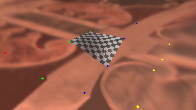
is the point on the surface that you get after you plug in the parameters. u and v are the parameters to the surface and should be within the range 0 to 1. These are the same thing as the t you see in Bezier curves, but there are two of them since there are two axes.

There are two Sigmas (summations) which mean that it’s a double for loop.

One of the for loops make i go from 0 to n and the other makes j go from 0 to m. m and n are the degree of each axis.

B_i^n(u) and B_i^n(u) are Bernstein polynomials (aka binomial expansion terms) just as you see in Bezier Curves – there is just one per axis.

Lastly comes the control points \mathbf{k}_{i,j}. The number of control on one axis are multiplied by the number of control points on the other axis.

A biquadratic Bezier patch has a degree of (2,2) and has 3 control points on one axis, and 3 control points on the other. That means that it has 9 control points total.

A bicubic Bezier patch has a degree of (3,3) with 4 control points on each axis, for a total of 16 control points.

If you had a patch of degree (7,1), it would have 8 control points on one axis and 2 control points on the other axis, and so would also have 16 control points total, but they would be laid out differently than a bicubic Bezier patch.

As far as actually calculating points on a curve, the above only calculates the value for a single axis for the final point on the curve. If you have three dimensional control points (X,Y,Z), you have to do the above math for each one to get the final result. This is the same as how it works for evaluating Bezier curves.

Code

#include 
#include 

typedef std::array TFloat3;
typedef std::array TFloat3x3;

const TFloat3x3 c_ControlPointsX =
{
    {
        { 0.7f, 0.8f, 0.9f },
        { 0.2f, 0.5f, 0.4f },
        { 0.6f, 0.3f, 0.1f },
    }
};

const TFloat3x3 c_ControlPointsY =
{
    {
        { 0.2f, 0.8f, 0.5f },
        { 0.6f, 0.9f, 0.3f },
        { 0.7f, 0.1f, 0.4f },
    }
};

const TFloat3x3 c_ControlPointsZ =
{
    {
        { 0.6f, 0.5f, 0.3f },
        { 0.7f, 0.1f, 0.9f },
        { 0.8f, 0.4f, 0.2f },
    }
};

void WaitForEnter ()
{
    printf("Press Enter to quit");
    fflush(stdin);
    getchar();
}

float QuadraticBezier (const TFloat3& p, float t)
{
    float s = 1.0f - t;
    float s2 = s * s;
    float t2 = t * t;

    return
        p[0] * s2 +
        p[1] * 2.0f * s * t +
        p[2] * t2;
}

float BiquadraticBezierPatch(const TFloat3x3& p, float u, float v)
{
    TFloat3 uValues;
    uValues[0] = QuadraticBezier(p[0], u);
    uValues[1] = QuadraticBezier(p[1], u);
    uValues[2] = QuadraticBezier(p[2], u);
    return QuadraticBezier(uValues, v);
}

int main(int argc, char **argv)
{
    // how many values to display on each axis. Limited by console resolution!
    const int c_numValues = 4;

    printf("Bezier rectangle:n");
    for (int i = 0; i < c_numValues; ++i)
    {
        float iPercent = ((float)i) / ((float)(c_numValues - 1));
        for (int j = 0; j < c_numValues; ++j)
        {
            if (j == 0)
                printf("  ");
            float jPercent = ((float)j) / ((float)(c_numValues - 1));
            float valueX = BiquadraticBezierPatch(c_ControlPointsX, jPercent, iPercent);
            float valueY = BiquadraticBezierPatch(c_ControlPointsY, jPercent, iPercent);
            float valueZ = BiquadraticBezierPatch(c_ControlPointsZ, jPercent, iPercent);
            printf("(%0.2f, %0.2f, %0.2f) ", valueX, valueY, valueZ);
        }
        printf("n");
    }
    printf("n");

    WaitForEnter();
    return 0;
}

And here is the output it gives:

Note that in the program above, I evaluate the surface points by evaluating one axis and then the other. This is basically the same as how I explained it at the top, where I’m effectively animating the control points over distance, then evaluating the curve slice of the surface at that specific distance.

You could also write it another way though, where you literally expand the mathematical formula to get just one expression to evaluate that takes all control points at once. I like the simplicity (of understanding) of the method I used, but the other method works just as well.

The Rendering

It’s easy enough to calculate values on a Bezier Rectangle, but what if you want to draw one?

One way is to tessellate it, or break it up into triangles and then render the triangles. You can think of it like trying to render a grid, where each point of the grid is moved to be where ever the Bezier rectangle function says it should be.

Raytracing against these objects in the general case is very difficult however, because it basically comes down to solving equations of very high degree.

Raymarching against these objects is also difficult unfortunately because while raymarching only needs to know “am i above the shape, or underneath it?”, knowing what u,v to plug into the equation to get the height most relevant to a random point in space is also very difficult. Not as difficult as the raytracing equations, but probably just as much out of reach.

But never fear, as always, you can cheat!

If you read my post about one dimensional (explicit) Bezier curves (One Dimensional Bezier Curves), you may remember that math gets easier if you use one dimensional control points. The same is actually true with Bezier rectangles!

For the ray marching case, you can march a point through space, and plug the x,z coordinate of the point into the Bezier rectangle function as u,v values and the number that comes out you can treat as a y coordinate.

Now, ray marching a Bezier rectangle is the same as ray marching any old height map (check links section for more info on that).

What I did in my demos, is since i knew that the curve was constrained to 0-1 on the x and z axis, and the y axis min and max was the control point min and maxes, I did a raytrace of that bounding box to get a minimum and maximum distance that the ray was inside that box. From there, I did raymarching from that min time to the max time along the ray, considering the ray as hitting the surface whenever the distance from the ray to the surface on the y axis (rayPos.y – bezierRectangle.y) changed sign.

After I had a hit, I got the height of the curve slightly offset on the x axis, then slightly offset on the z axis to get a triangle that I could calculate a surface normal from, to do lighting and shading with.

There is room for improvement in the ray marching though. I evenly divide the space through the box by a specific amount to control the size of the steps. A better way to do this I think would be to get the gradient of the function and use that to get a distance estimate (check links section below for more information). I could use that value to control the distance the ray marches at each step, and should be able to march through the box much quicker.

Also, as the link on terrain marching explains, you can usually take farther steps when the ray is farther from the camera, because the eye notices less detail. I removed that since the Bezier rectangles are pretty close to the camera, but it probably still would be helpful. Also, it would DEFINITELY be helpful in the case of the “Infinite Bezier Rectangles” scene.

I am pretty sure you could directly raytrace an explicit Bezier rectangle (one who has one dimensional control points) – at least for low degrees. I personally don’t know how you would do that, but I think it might boil down to solving a 4th degree function or something else “reasonable” based on a similar question I had about Bezier triangles on the mathematics stack exchange site (link below).

Another Way To Render

There is another way to render Bezier surfaces using ray based methods that I didn’t use but want to mention.

A property of Bezier curves and surfaces is that they are guaranteed to be completely contained by the convex hull created by their control points.

Another property of Bezier curves and surfaces is that you can use the De Casteljeau algorithm to cut them up. For instance you could cut a Bezier curve into two different Bezier curves, and the same holds for Bezier surfaces.

Using these two properties, there is an interesting way to be able to tell if a ray intersects a bezier curve or not, which is:

  1. If the line misses the convex hull, return a miss
  2. If the convex hull is smaller than a pixel, return a hit
  3. Otherwise, cut the Bezier object into a couple smaller Bezier objects
  4. Recurse for each smaller Bezier object

Yes, believe it or not, that is a real technique! It’s called Bezier Clipping and there is a research paper in the links section below that talks about some of the details of using that rendering technique.

Links

Lastly, I wanted to mention that the above is completely about Bezier rectangles, but there is no reason you couldn’t extend these rectangles to use rational Bezier functions, or be based on B-splines or NURBS, or even go a different direction and make hermite surfaces or catmull-rom surfaces, or even make surfaces that used exotic basis functions of your own crafting based on trigonometric functions or whatever else!

Here are the shadertoy demos I made:
Shadertoy: Cubic Bezier Rectangle
Shadertoy: Quadratic Bezier Rectangle
Shadertoy: Infinite Bezier Rectangles

And some other links about this stuff:
IQ – terrain raymarching
IQ – distance estimation (using function gradients)
Math Stack Exchange – Ray intersection with explicit (1 axis) Bezier triangle?
Math Stack Exchange – Intersect Ray (Line) vs Quadratic Bezier Triangle
Bézier Surfaces: de Casteljau’s Algorithm
Ray Tracing Triangular Bézier Patches (including Bezier clipping)
Wikipedia: Bezier Surface
Wikipedia: Bezier Triangle