Bresenham’s Drawing Algorithms

If you were asked to name a line drawing algorithm, chances are you would say Bresenham. I recently needed to write my own software line drawing algorithm (CPU and regular ram, not GPU and VRAM) and Bresenham was the first to come to mind for me as well.

Believe it or not, Jack Bresenham actually came up with 2 famous line drawing algorithms. One is a run length algorithm, and the other is a run slice algorithm. People are most often familiar with the run length algorithm, which I mainly talk about in this post, but there’s some information about the run slice algorithm and links to other Bresenham primitive rendering algorithms below as well!

An interesting thing about both line algorithms is that they involve only integer mathematics, so there is no round off error, epsilons, numerical instability or anything like that. You use only integers and simple math (no divisions even!), and get the exact right answer out. I think that is pretty cool.

Bresenham’s Run Length Line Algorithm Summarized

To help understand the code, I want to give a brief summarization of how the algorithm works at a high level.

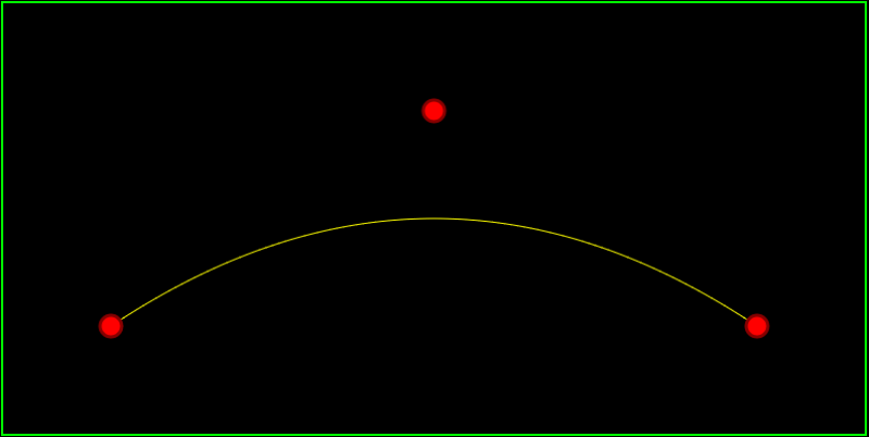
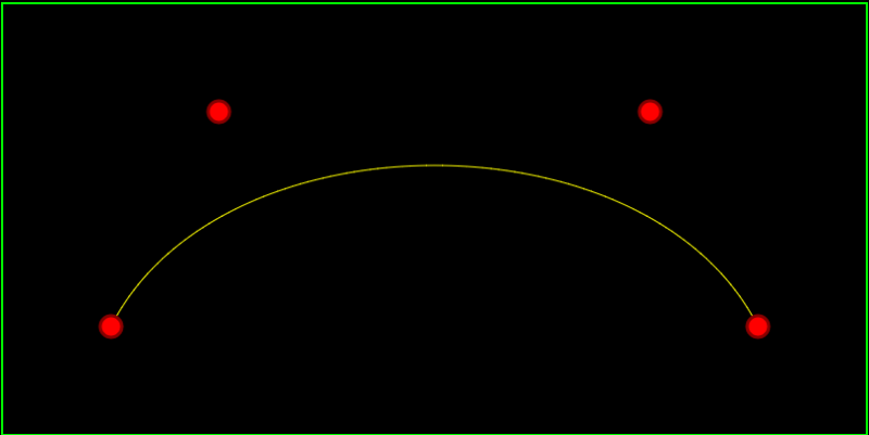
The first step of the Bresenham line algorithm is to see if the line is longer on the X axis or Y axis. Whichever one it is longer on is the major axis, and the shorter one is the minor axis.

Then, starting at the starting point of the line, you loop across all pixels of the major axis, doing some math to decide for each pixel whether you need to move the pixel on the minor axis yet or not. Basically you keep track of the error – or the distance the pixel is away from the true position of the line on the minor axis – and if the error is greater than or equal to 1 pixel, you move the pixel on the minor axis and subtract one pixel from the error. If the error is smaller than 1 pixel, you keep it at the same value it was for the last pixel, and keep the error value the same, so that it can accumulate some more error for the next pixel and test again.


The left line is longer on the X axis, so the major axis is the X axis. The right line is longer on the Y axis, so the major axis is the Y axis. Notice that there is one pixel for each value along the major axis of each line, but repeated pixel values along the minor axis of each line.

If you want the deeper details about the algorithm or the math behind it, check out this link:
Wikipedia: Bresenham’s line algorithm

One Octant Code

Wikipedia says that many implementations implement the algorithm for a single octant (half of a quadrant) and then use coordinate conversions (flipping the x and y’s and/or negating them) to make the same logic work for any quadrant.

In that vein, here is a simple implementation for the first octant – where the major axis is X, and both X and Y are increasing from the starting point to the ending point.

	void DrawLine (int x1, int y1, int x2, int y2, unsigned int color)
	{
		const int dx = x2 - x1;
		const int dy = y2 - y1;

		int Error = 2 * dy - dx;
		int y = y1;
		
		DrawPixel(x1, y1, color);
		for (int x = x1+1; x < x2; ++x)
		{
			if (Error > 0)
			{
				y++;
				Error += 2 * dy - 2 * dx;
			}
			else
			{
				Error += 2 * dy;
			}
			DrawPixel(x,y,color);
		}
	}

With the point of Bresenham being that it is efficient, let’s sacrifice readability a bit and get rid of those DrawPixel calls and perhaps over-micro-optimize a bit and make some consts for frequently used values.

	void DrawLine (unsigned int* pixels, int width, int x1, int y1, int x2, int y2, unsigned int color)
	{
		const int dx = x2 - x1;
		const int dy = y2 - y1;
		const int dx2 = dx * 2;
		const int dy2 = dy * 2;
		const int dy2Mindx2 = dy2 - dx2;

		int Error = dy2 - dx;

		unsigned int* pixel = &amp;pixels[y1*width+x1];
		*pixel = color;
		for (int x = x2 - x1 - 1; x > 0; --x)
		{
			if (Error > 0)
			{
				pixel += width + 1;
				Error += dy2Mindx2;
			}
			else
			{
				pixel++;
				Error += dy2;
			}
			*pixel = color;
		}
	}

Cool, now let’s make it work for any line.

Final Code

	// Generic Line Drawing
	// X and Y are flipped for Y maxor axis lines, but the pixel writes are handled correctly due to
	// minor and major axis pixel movement
	void DrawLineMajorAxis(
		unsigned int* pixel,
		int majorAxisPixelMovement,
		int minorAxisPixelMovement,
		int dx,
		int dy,
		unsigned int color
	)
	{
		// calculate some constants
		const int dx2 = dx * 2;
		const int dy2 = dy * 2;
		const int dy2Mindx2 = dy2 - dx2;

		// calculate the starting error value
		int Error = dy2 - dx;

		// draw the first pixel
		*pixel = color;

		// loop across the major axis
		while (dx--)
		{
			// move on major axis and minor axis
			if (Error > 0)
			{
				pixel += majorAxisPixelMovement + minorAxisPixelMovement;
				Error += dy2Mindx2;
			}
			// move on major axis only
			else
			{
				pixel += majorAxisPixelMovement;
				Error += dy2;
			}

			// draw the next pixel
			*pixel = color;
		}
	}

	// Specialized Line Drawing optimized for horizontal or vertical lines
	// X and Y are flipped for Y maxor axis lines, but the pixel writes are handled correctly due to
	// minor and major axis pixel movement
	void DrawLineSingleAxis(unsigned int* pixel, int majorAxisPixelMovement, int dx, unsigned int color)
	{
		// draw the first pixel
		*pixel = color;

		// loop across the major axis and draw the rest of the pixels
		while (dx--)
		{
			pixel += majorAxisPixelMovement;
			*pixel = color;
		};
	}

	// Draw an arbitrary line.  Assumes start and end point are within valid range
	// pixels is a pointer to where the pixels you want to draw to start aka (0,0)
	// pixelStride is the number of unsigned ints to get from one row of pixels to the next.
	// Usually, that is the same as the width of the image you are drawing to, but sometimes is not.
	void DrawLine(unsigned int* pixels, int pixelStride, int x1, int y1, int x2, int y2, unsigned int color)
	{
		// calculate our deltas
		int dx = x2 - x1;
		int dy = y2 - y1;

		// if the X axis is the major axis
		if (abs(dx) >= abs(dy))
		{
			// if x2 < x1, flip the points to have fewer special cases
			if (dx < 0)
			{
				dx *= -1;
				dy *= -1;
				swap(x1, x2);
				swap(y1, y2);
			}

			// get the address of the pixel at (x1,y1)
			unsigned int* startPixel = &amp;pixels[y1 * pixelStride + x1];

			// determine special cases
			if (dy > 0)
				DrawLineMajorAxis(startPixel, 1, pixelStride, dx, dy, color);
			else if (dy < 0)
				DrawLineMajorAxis(startPixel, 1, -pixelStride, dx, -dy, color);
			else
				DrawLineSingleAxis(startPixel, 1, dx, color);
		}
		// else the Y axis is the major axis
		else
		{
			// if y2 < y1, flip the points to have fewer special cases
			if (dy < 0)
			{
				dx *= -1;
				dy *= -1;
				swap(x1, x2);
				swap(y1, y2);
			}

			// get the address of the pixel at (x1,y1)
			unsigned int* startPixel = &amp;pixels[y1 * pixelStride + x1];

			// determine special cases
			if (dx > 0)
				DrawLineMajorAxis(startPixel, pixelStride, 1, dy, dx, color);
			else if (dx < 0)
				DrawLineMajorAxis(startPixel, pixelStride, -1, dy, -dx, color);
			else
				DrawLineSingleAxis(startPixel, pixelStride, dy, color);
		}
	}

Using the above functions, I wrote a little test to draw lines from the center of an image towards the edges at 100 different angles, and also a horizontal and vertical line. Here’s the results:

Run Slice Algorithm

So, like I said above, there is another Bresenham line algorithm that is a run slice algorithm.

What that means is that instead of looping across the major axis figuring out if each pixel needs to move on the minor axis as well, instead it loops across the minor axis, figuring out how many pixels it needs to write for that row or column of pixels.

One benefit of that algorithm is that it is less loop iterations since it’s looping across the minor axis pixels instead of the major axis.

Here’s an interesting read about Michael Abrash and his encounters with and the run slice algorithm:

Michael Abrash’s Graphics Programming Black Book Special Edition: The Good, the Bad, and the Run-Sliced

Other Bresenham Algorithms

This was origionally just going to be about the line algorithms, and I was going to make up another post about the circle algorithm, but I changed my mind.

While doing some research to see if there was a Bresenham bezier curve algorithm I stumbled on the page below, which shows that yes, there is! There are quite a few other algorithms as well:

Many Bresenham algorithms with very short c++ implementations

Dual Numbers & Automatic Differentiation

In the last post, I talked about imaginary numbers, complex numbers, and how to use them to rotate vectors in 2d.

In this post, I want to share another interesting type of number called a “Dual Number” that uses the symbol ε (epsilon) and has a neat trick of automatically calculating the derivative of a function while you calculate the value of the function at the same time.

Dual numbers are pretty similar to imaginary numbers but there is one important difference. With imaginary numbers, i^2 = -1, but with dual numbers, ε^2 = 0 (and ε is not 0!). That may seem like a small difference, but oddly, that opens up a whole interesting world of mathematical usefulness.

Before we dig into automatic differentiation, I want to go over the mathematical basics for how dual numbers behave.

Basic Dual Number Math

Adding dual numbers is the same as adding complex numbers; you just add the real and dual parts separately:

(3 + 4ε) + (1 + 2ε) = 4 + 6ε

Subtraction works the same way as well:

(3 + 4ε) – (1 + 2ε) = 2 + 2ε

To multiply dual numbers, you use F.O.I.L. just like you do with complex numbers:

(3 + 4ε) * (1 + 2ε) =
3 + 6ε + 4ε + 8ε^2 =
3 + 10ε + 8ε^2

However, since ε^2 is zero, the last term 8ε^2 disappears:
3 + 10ε

It’s interesting to note that with complex numbers, the i^2 became -1, so the last term changed from imaginary to real, meaning that the imaginary numbers fed back into the real numbers during multiplication. With dual numbers, that isn’t the case, the dual numbers don’t feed back into the real numbers during multiplication.

In both complex and dual numbers the real terms do affect the non real terms during multiplication.

The division operator relates to the conjugate. I have source code for it below, and some of the links at the end of the post go into the details of that and other operations.

Quick Review: Derivatives (Slope)

If you know the line formula y=mx+b, but you don’t know what a derivative is you are in luck. Remember how “m” is the slope of the line, specifying how steep it is? That is what the derivative is too, it’s just the slope.

Below is a graph of y=2x+1. At every point on that line, the derivative (or slope) is 2. That means that for every step we make on the x axis to the right (positive direction), we make 2 steps up on the y axis (positive direction).

Now, check out this graph of y=x^2-0.2

The derivative (or slope) at every point on this graph is 2x. That means that the slope changes depending on where the x coordinate is!

So, when x=0, the slope is 0. You can see that in the graph where x=0, that it is horizontal, meaning that a step on the x axis becomes no steps on the y axis (only at that point where x is 0, and only if you take an infinitely small step).

When x is 1, the slope is 2, when x is 2, the slope is 4, when x is 3, the slope is 6. Since the numbers increase as we increase x from 0, that tells us that the graph gets steeper as we go to the right, which you can see in the graph.

Alternately, when x is -1, the slope is -2, when x is -2, the slope is -4, and when x is -3, the slope is -6. This shows us that as we decrease x from 0, the graph gets steeper in the opposite direction, which you can see in the graph as well.

What is Automatic Differentiation?

Let’s say you have a function (possibly a curve) describing the path of a rocket, and you want to make the rocket point down the path that it’s traveling.

One way you might do this is to evaluate your function f(T) to get the current location of your rocket (where T is how long the rocket has been flying), and then calculate the derivative f'(T) to find the slope of the graph at that point so that you can orient the rocket in that direction.

You could calculate the value and slope of the function at time T independently easily enough if you know how to get the derivative of a function (a calculus topic), or use wolframalpha.com.

However, if you have a complex equation, or maybe if the equation is controlled by user input, or game data, it might not be so easy to figure out what the derivative is at run time.

For instance… imagine having a function that rolled random numbers to figure out what mathematical operation it should preform on a number next (if we roll a 0, add 3, if we roll a 1 multiply by 2, if we roll a 2, square the number… etc). It isn’t going to be simple to take the derivative of the same mathematical function.

Here enters automatic differentiation (or AD). AD lets you calculate the derivative WHILE you are calculating the value of the function.

That way, you can do whatever math operations you want on your number, and in the end you will have both the value of f(T) as well as the derivative f'(T).

Using ε for Automatic Differentiation

You can use dual number operations on numbers to calculate the value of f(x) while also calculating f'(x) at the same time. I’ll show you how with a simple example using addition and multiplication like we went over above.

We’ll start with the function f(x)=3x+2, and calculate f(4) and f'(4).

the first thing we do is convert our 4 into a dual number, using 1 for the dual component, since we are plugging it in for the value of x, which has a derivative of 1.

4+1ε

Next, we want to multiply that by the constant 3, using 0 for the dual component since it is just a constant (and the derivative of a constant is 0)

(4+1ε) * (3 + 0ε) =
12 + 0ε + 3ε + 0ε^2 =
12 + 3e

Lastly, we need to add the constant 2, using 0 again for the dual component since it’s just a constant.
(12 + 3ε) + (2 + 0ε) =
14 + 3ε

In our result, the real number component (14) is the value of f(4) and the dual component (3) is the derivative f'(4), which is correct if you work it out!

Let’s try f(5). First we convert 5 to a dual number, with the dual component being 1.

5 + 1ε

Next we need to multiply it by the constant 3 (which has a dual component of 0)

(5 + 1ε) * (3 + 0e) =
15 + 0ε + 3ε + 0ε^2 =
15 + 3ε

Now, we add the constant 2 (which has a dual component of 0 again since it’s just a constant)
(15 + 3ε) + (2 + 0ε) =
17 + 3ε

So, our answer says that f(5) = 17, and f'(5) = 3, which again you can verify is true!

Quadratic Example

The example above worked well but it was a linear function. What if we want to do a function like f(x) = 5x^2 + 4x + 1?

Let’s calculate f(2). We are going to first calculate the 5x^2 term, so we need to start by making a dual number for the function parameter x:
(2 + 1ε)

Next, we need to multiply it by itself to make x^2:
(2 + 1ε) * (2 + 1ε) =
4 + 2ε + 2ε + 1ε^2 =
4 + 4ε

(remember that ε^2 is 0, so the last term disappears)

next, we multiply that by the constant 5 to finish making the 5x^2 term:
(4 + 4ε) * (5 + 0ε) =
20 + 0ε + 20ε + 0ε^2 =
20 + 20ε

Now, putting that number aside for a second we need to calculate the “4x” term by multiplying the value we plugged in for x by the constant 4
(2 + 1ε) * (4 + 0ε) =
8 + 0ε + 4ε + 0ε^2 =
8 + 4ε

Next, we need to add the last 2 values together (the 5x^2 term and the 4x term):
(20 + 20ε) + (8 + 4ε) =
28 + 24ε

Lastly, we need to add in the last term, the constant 1
(28 + 24ε) + (1 + 0ε) =
29 + 24e

There is our answer! For the equation y = 5x^2 + 4x + 1, f(2) = 29 and f'(2) = 24. Check it, it’s correct (:

As one last example let’s calculate f(10) and f'(10) with the same function above y = 5x^2 + 4x + 1.

First, to start calculating the 5x^2 term, we need to make 10 into a dual number and multiply it by itself to make x^2:
(10 + 1ε) * (10 + 1ε) =
100 + 10ε + 10ε + 1ε^2 =
100 + 20ε

Next, we multiply by the constant 5 to finish making the 5x^2 term:
(100 + 20ε) * (5 + 0ε) =
500 + 0ε + 100ε + 0ε^2 =
500 + 100ε

Putting that aside, let’s calculate the 4x term by multiplying our x value by the constant 4:
(10 + 1ε) * (4 + 0ε) =
40 + 0ε + 4ε + 0ε^2 =
40 + 4ε

Lastly, let’s add our terms: 5x^2, 4x and the constant 1
(500 + 100ε) + (40 + 4ε) + (1 + 0ε) =
541 + 104ε

The answer tells us that for the equation y = 5x^2 + 4x + 1, f(10) = 541 and f'(10) = 104.

Sample Code

There are lots of other mathematical operations that you can do with dual numbers. I’ve collected as many as I was able to find and made up some sample code that uses them. The sample code is below, as well as the program output.

#include 
#include 

#define PI 3.14159265359f

// In production code, this class should probably take a template parameter for
// it's scalar type instead of hard coding to float
class CDualNumber
{
public:
	CDualNumber (float real = 0.0f, float dual = 0.0f)
		: m_real(real)
		, m_dual(dual)
	{
	}

	float Real () const { return m_real; }
	float Dual () const { return m_dual; }

private:
	float m_real;
	float m_dual;
};

//----------------------------------------------------------------------
// Math Operations
//----------------------------------------------------------------------
inline CDualNumber operator + (const CDualNumber &a, const CDualNumber &b)
{
	return CDualNumber(a.Real() + b.Real(), a.Dual() + b.Dual());
}

inline CDualNumber operator - (const CDualNumber &a, const CDualNumber &b)
{
	return CDualNumber(a.Real() - b.Real(), a.Dual() - b.Dual());
}

inline CDualNumber operator * (const CDualNumber &a, const CDualNumber &b)
{
	return CDualNumber(
		a.Real() * b.Real(),
		a.Real() * b.Dual() + a.Dual() * b.Real()
	);
}

inline CDualNumber operator / (const CDualNumber &a, const CDualNumber &b)
{
	return CDualNumber(
		a.Real() / b.Real(),
		(a.Dual() * b.Real() - a.Real() * b.Dual()) / (b.Real() * b.Real())
	);
}

inline CDualNumber sqrt (const CDualNumber &a)
{
	float sqrtReal = ::sqrt(a.Real());
	return CDualNumber(
		sqrtReal,
		0.5f * a.Dual() / sqrtReal
	);
}

inline CDualNumber pow (const CDualNumber &a, float y)
{
	return CDualNumber(
		::pow(a.Real(), y),
		y * a.Dual() * ::pow(a.Real(), y - 1.0f)
	);
}

inline CDualNumber sin (const CDualNumber &a)
{
	return CDualNumber(
		::sin(a.Real()),
		a.Dual() * ::cos(a.Real())
	);
}

inline CDualNumber cos (const CDualNumber &a)
{
	return CDualNumber(
		::cos(a.Real()),
		-a.Dual() * ::sin(a.Real())
	);
}

inline CDualNumber tan (const CDualNumber &a)
{
	return CDualNumber(
		::tan(a.Real()),
		a.Dual() / (::cos(a.Real()) * ::cos(a.Real()))
	);
}

inline CDualNumber atan (const CDualNumber &a)
{
	return CDualNumber(
		::atan(a.Real()),
		a.Dual() / (1.0f + a.Real() * a.Real())
	);
}

inline CDualNumber SmoothStep (CDualNumber x)
{
	// f(x) = 3x^2 - 2x^3
	// f'(x) = 6x - 6x^2
	return x * x * (CDualNumber(3) - CDualNumber(2) * x);
}

//----------------------------------------------------------------------
// Test Functions
//----------------------------------------------------------------------

void TestSmoothStep (float x)
{
	CDualNumber y = SmoothStep(CDualNumber(x, 1.0f));
	printf("smoothstep 3x^2-2x^3(%0.4f) = %0.4fn", x, y.Real());
	printf("smoothstep 3x^2-2x^3'(%0.4f) = %0.4fnn", x, y.Dual());
}

void TestTrig (float x)
{
	CDualNumber y = sin(CDualNumber(x, 1.0f));
	printf("sin(%0.4f) = %0.4fn", x, y.Real());
	printf("sin'(%0.4f) = %0.4fnn", x, y.Dual());

	y = cos(CDualNumber(x, 1.0f));
	printf("cos(%0.4f) = %0.4fn", x, y.Real());
	printf("cos'(%0.4f) = %0.4fnn", x, y.Dual());

	y = tan(CDualNumber(x, 1.0f));
	printf("tan(%0.4f) = %0.4fn", x, y.Real());
	printf("tan'(%0.4f) = %0.4fnn", x, y.Dual());

	y = atan(CDualNumber(x, 1.0f));
	printf("atan(%0.4f) = %0.4fn", x, y.Real());
	printf("atan'(%0.4f) = %0.4fnn", x, y.Dual());
}

void TestSimple (float x)
{
	CDualNumber y = CDualNumber(3.0f) / sqrt(CDualNumber(x, 1.0f));
	printf("3/sqrt(%0.4f) = %0.4fn", x, y.Real());
	printf("3/sqrt(%0.4f)' = %0.4fnn", x, y.Dual());

	y = pow(CDualNumber(x, 1.0f) + CDualNumber(1.0f), 1.337f);
	printf("(%0.4f+1)^1.337 = %0.4fn", x, y.Real());
	printf("(%0.4f+1)^1.337' = %0.4fnn", x, y.Dual());
}

int main (int argc, char **argv)
{
	TestSmoothStep(0.5f);
	TestSmoothStep(0.75f);
	TestTrig(PI * 0.25f);
	TestSimple(3.0f);
	return 0;
}

Here is the program output:

Closing Info

When you are thinking what number ε has to be so that ε^2 is 0 but ε is not 0, you may be tempted to think that it is an imaginary number, just like i (the square root of -1) that doesn’t actually exist. This is actually not how it is… I’ve seen ε described in two ways.

One way I’ve seen it described is that it’s an infinitesimal number. That sort of makes sense to me, but not in a concrete and tangible way.

The way that makes more sense to me is to describe it as a matrix like this:
[0, 1]
[0, 0]

If you multiply that matrix by itself, you will get zero(s) as a result.

In fact, an alternate way to implement the dual numbers is to treat them like a matrix like that.

I also wanted to mention that it’s possible to modify this technique to get the 2nd derivative of a function or the 3rd, or the Nth. It isn’t only limited to the 1st derivative. Check the links at the bottom of this post for more info, but essentially, if you want 1st and 2nd derivative, you need to make it so that ε^3 = 0 instead of ε^2 = 0. There is a way to do that with matrices.

Another neat thing is that you can also extend this into multiple dimensions. This is useful for situations like if you have some terrain described by mathematical functions, when you are walking the grid of terrain to make vertex information, you can get the slope / gradient / surface normal at the same time.

Lastly, I wanted to mention a different kind of number called a hyperbolic number.

The imaginary number i^2 = -1 and we can use it to do 2d rotations.

The dual number ε^2 is 0 (and ε is not 0) and we can use it to do automatic differentiation.

Hyperbolic numbers have j, and j^2 = 1 (and j is not 1). I’m not sure, but I bet they have some interesting usefulness to them too. It would be interesting to research that more sometime. If you know anything about them, please post a comment!

Links

This shadertoy is what got me started looking into dual numbers. It’s a mandelbrot viewer done by iq using dual numbers to estimate a distance from a point to the mandelbrot set (as far as I understand it anyhow, ha!). He uses that estimated distance to color the pixels.

Shadertoy: Dual Complex Numbers

I didn’t get very much into the reasons of why this works (has to do with taylor series terms disappearing if ε^2 is 0), or the rigorous math behind deriving the operators, but here are some great links I found researching this stuff and putting this blog post together.

Wikipedia: Dual Number
[Book] Dual-Number Methods in Kinematics, Statics and Dynamics By Ian Fischer
[GDC2012] Math for Game Programmers: Dual Numbers by Gino van den Bergen
Stackexchange: Implementing trig functions for dual numbers
Exact numeric nth derivatives
Automatic Differentiation with Dual numbers
Wikipedia: Automatic Differentiation

Four Ways to Calculate Sine Without Trig

Is it possible to sin without trig? That is a question that has plagued theologians for centuries. As evil as trigonometry is, modern science shows us that yes, it is possible to sin without trig. Here are some ways that I’ve come across.

1 – Slope Iteration Method


The above image uses 1024 samples from 0 to 2pi to aproximate sine iteratively using it’s slope. Red is true sin, green is the aproximation, and yellow is where they overlap.

This method comes from Game Programming Gems 8, which you can snag a copy of from amazon below if you are interested. It’s mentioned in chapter 6.1 A Practical DSP Radio Effect (which is a really cool read btw!).
Amazon: Game Programming Gems 8

This method uses calculus but is actually pretty straightforward and intuitive – and very surprising to me that it works so well!

The derivative of sin(x) is cos(x). That means, for any x you plug into sin, the slope of the function at that point is the cosine value of that same x.

In other words, sin(0) is 0, but it has a slope of cos(0) which is 1. Since slope is rise over run (change in y / change in x) that means that at sin(0), if you take an infinitely small step forward on x, you need to take the same sized step on y. That will get you to the next value of sine.

Let’s test that out!
sin(0) = 0 so we start at (0,0) on the graph.

If we try a step size of 0.1, our approximation is:
sin(0.1) = 0.1

The actual value according to google is 0.09983341664. so our error was about 0.0002. That is actually pretty close!

How about 0.25?
sin(0.25) = 0.25

The real value is 0.24740395925, so our error is about 0.003. We have about 10 times the error that we did at 0.1.

what if we try it with 0.5?
sin(0.5) = 0.5

The actual value is 0.4794255386, which leaves us with an error of about 0.02. Our error is 100 times as much as it was at 0.1. As you can see, the error increases as our step size gets larger.

If we wanted to, we could get the slope (cosine value) at the new x value and take another step. we could continue doing this to get our sine approximation, knowing that the smaller the step that we use, the more accurate our sine approximation would be.

We haven’t actually won anything at this point though, because we are just using cosine to take approximated steps through sine values. We are paying the cost of calculating cosine, so we might as well just calculate sine directly instead.

Well luckily, cosine has a similar relationship with sine; the derivative of cos(x) is -sin(x).

Now, we can use cosine values to step through sine values, and use those same sine values to step through cosine values.

Since we know that cos(0) = 1.0 and sin(0) = 0.0, we can start at an angle of 0 with those values and we can iteratively step through the values.

Here is a sample function in C++

// theta is the angle we want the sine value of.
// higher resolution means smaller step size AKA more accuracy but higher computational cost.
// I used a resolution value of 1024 in the image at the top of this section.
float SineApproximation (float theta, float resolution)
{
    // calculate the stepDelta for our angle.
    // resolution is the number of samples we calculate from 0 to 2pi radians
    const float TwoPi = 6.28318530718f;
    const float stepDelta = (TwoPi / resolution);

    // initialize our starting values
    float angle = 0.0;
    float vcos = 1.0;
    float vsin = 0.0;

    // while we are less than our desired angle
    while(angle < theta) {

        // calculate our step size on the y axis for our step size on the x axis.
        float vcosscaled = vcos * stepDelta;
        float vsinscaled = vsin * stepDelta;

        // take a step on the x axis
        angle += stepDelta;

        // take a step on the y axis
        vsin += vcosscaled;
        vcos -= vsinscaled;
    }

    // return the value we calculated
    return vsin;
}

Note that the higher the angle you use, the more the error rate accumulates. One way to help this would be to make sure that theta was between 0 and 2pi, or you could even just calculate between 0 and pi/2 and mirror / reflect the values for the other quadrants.

This function is quite a bit of work to calculate a single value of sine but it’s real power comes in the fact that it’s iterative. If you ever find yourself in a situation where you need progressive values of sine, and have some fixed angle step size through the sine values, this algorithm just needs to do a couple multiplies and adds to get to the next value of sine.

One great use of this could be in DSP / audio synthesis, for sine wave generation. Another good use could be in efficiently evaluating trigonometry based splines (a future topic I plan to make a post about!).

You can see this in action in this shadertoy or look below at the screenshots:
Shadertoy: Sin without Trig

64 Samples – Red is true sine, green is our approximation, and yellow is where they are the same

128 Samples

256 Samples

1024 Samples

2 – Taylor Series Method

Another way to calculate sine is by using an infinite Taylor series. Thanks to my friend Yuval for showing me this method.

You can get the Taylor series for sine by typing “series sin(x)” into wolfram alpha. You can see that here: Wolfram Alpha: series sin(x).

Wolfram alpha says the series is: x-x^3/6+x^5/120-x^7/5040+x^9/362880-x^11/39916800 ….

what this means is that if you plug a value in for x, you will get an approximation of sine for that x value. It’s an infinite series, but you can do as few or as many terms as you want to be able to trade off speed for accuracy.

For instance check out these graphs.

Google: graph y = x, y = sin(x)

Google: graph y = x-x^3/6, y = sin(x)

Google: graph y = x-x^3/6+x^5/120, y = sin(x)

Google: graph y = x-x^3/6+x^5/120-x^7/5040, y = sin(x)

Google: graph y = x-x^3/6+x^5/120-x^7/5040+x^9/362880, y = sin(x)

Google: graph y = x-x^3/6+x^5/120-x^7/5040+x^9/362880-x^11/39916800, y = sin(x)
(Note that I had to zoom out a bit to show where it became inaccurate)

When looking at these graphs, you’ll probably notice that very early on, the approximation is pretty good between -Pi/2 and + Pi/2. I leveraged that by only using those values (with modulus) and mirroring them to be able to get a sine value of any angle with more accuracy.

When using just x-x^3/6, there was an obvious problem at the top and bottom of the sine waves:

When i boosted the equation with another term, bringing it to x-x^3/6+x^5/120, my sine approximation was much better:

You can see this method in action in this shadertoy:
Shadertoy: Sin without Trig II

3 – Smoothstep Method

The third method may be my favorite, due to it’s sheer elegance and simplicity. Thanks to P_Malin on shadertoy.com for sharing this one with me.

There’s a function in graphics called “smoothstep” that is used to take the hard linear edge off of things, and give it a smoother, more organic feel. You can read more about it here: Wikipedia: Smoothstep.

BTW if you haven’t read the last post, I talk about how smooth step is really just a 1d bezier curve with specific control points (One Dimensional Bezier Curves). Also, smoothstep is just this function: y = (3x^2 – 2x^3).

Anyhow, if you have a triangle wave that has values from 0 to 1 on the y axis, and put it through a smoothstep, then scale it to -1 to +1 on the y axis, you get a pretty darn good sine approximation out.

Here is a step by step recipe:

Step 1 – Make a triangle wave that has values on the y axis from 0 to 1

Step 2 – Put that triangle wave through smoothstep (3x^2 – 2x^3)

Step 3 – Scale the result to having values from -1 to +1 on the axis.

That is pretty good isn’t it?

You can see this in action in this shadertoy (thanks to shadertoy’s Dave_Hoskins for some help with improving the code):
Shadertoy: Sin without Trig III

After I made that shadertoy, IQ, the creator of shadertoy who is an amazing programmer and an impressive “demoscene” guy, said that he experimented with removing the error from that technique to try to get a better sin/cos aproximation.

You can see that here: Shadertoy: Sincos approximation

Also, I recommend checking out IQ’s website. He has a lot of interesting topics on there: IQ’s Website

4 – CORDIC Mathematics

This fourth way is a method that cheaper calculators use to calculate trig functions, and other things as well.

I haven’t taken a whole lot of time to understand the details, but it looks like it’s using imaginary numbers to rotate vectors iteratively, doing a binary search across the search space to find the desired values.

The benefit of this technique is that it can be implemented with VERY little hardware support.

The number of logic gates for the implementation of a CORDIC is roughly comparable to the number required for a multiplier as both require combinations of shifts and additions.
Wikipedia: Coordinate Rotation Digital Computer

Did I miss any?

If you know of something that I’ve left out, post a comment, I’d love to hear about it!

One Dimensional Bezier Curves

I was recently looking at the formula for bezier curves:

Quadratic Bezier curve:
A * (1-T)^2 + B * 2 * (1-T) * T + C * T ^2

Cubic Bezier curve:
A*(1-T)^3+3*B*(1-T)^2*T+3*C*(1-T)*T^2+D*T^3

(more info available at Bezier Curves Part 2 (and Bezier Surfaces))

And I wondered… since you can have a Bezier curve in any dimension, what would happen if you made the control points (A,B,C,D) scalar? In other words, what would happen if you made bezier curves 1 dimensional?

Well it turns out something pretty interesting happens. If you replace T with x, you end up with f(x) functions, like the below:

Quadratic Bezier curve:
y = A * (1-x)^2 + B * 2 * (1-x) * x + C * x ^2

Cubic Bezier curve:
y = A*(1-x)^3+3*B*(1-x)^2*x+3*C*(1-x)*x^2+D*x^3

What makes that so interesting is that most math operations you may want to do on a bezier curve are a lot easier using y=f(x), instead of the parameterized formula Point = F(S,T).

For instance, try to calculate where a line segment intersects with a parameterized bezier curve, and then try it again with a quadratic equation. Or, try calculating the indefinite integral of the parameterized curve so that you can find the area underneath it (like, for Analytic Fog Density). Or, try to even find the given Y location that the curve has for a specific X value. These things are pretty difficult with a parameterized function, but a lot easier with the y=f(x) style function.

This ease of use does come at a price though. Specifically, you can’t move control points freely, you can only move them up and down and cannot move them left and right. If you are ok with that trade off, these 1 dimensional curves can be pretty powerful.

Below is an image of a 1 dimensional cubic bezier curve that has control points A = 0.5 B = 0.25 C = 0.75 D = 0.5. The function of this curve is y = 0.5 * (1-x)^3 + 0.25 * 3x(1-x)^2 + 0.75 * 3x^2(1-x) + 0.5 * x^3.

You can ask google to graph that for you to see that it is in fact the same: Google: graph y = 0.5 * (1-x)^3 + 0.25 * 3x(1-x)^2 + 0.75 * 3x^2(1-x) + 0.5 * x^3

cubicbez

Another benefit to these one dimensional bezier curves is that you could kind of use them as a “curve fitting” method. If you have some data that you wanted to approximate with a quadratic function, you could adjust the control points of a one dimensional quadratic Bezier curve to match your data set. If you need more control points to get a better aproximation of the data, you can just increase the degree of the bezier curve (check this out for more info on how to do that: Bezier Curves Part 2 (and Bezier Surfaces)).

Smoothstep as a Cubic 1d Bezier Curve

BIG THANKS to CeeJay.dk for telling me about this, this is pretty rad.

It’s kind of out of the scope of this post to talk about why smoothstep is awesome, but to give you strong evidence that it is, it’s a GLSL built in function. You may have also seen it used in the post I made about distance fields (Distance Field Textures), because one of it’s common uses is to make the edges of things look smoother. Here’s a wikipedia page on it as well if you want more info: Wikipedia: Smoothstep

Anyhow, I had no idea, but apparently the smoothstep equation is the same as if you take a 1d cubic bezier curve and make the first two control points 0, and the last two control points 1.

The equation for smoothstep is: y = 3*x^2 – 2*x^3

The equation for the bezier curve i mentioned is: y = 0*(1-x)^3+3*0*(1-x)^2*x+3*1*(1-x)*x^2+1*x^3

otherwise known as: y = 3*1*(1-x)*x^2+1*x^3

If you work it out, those are the same equations! Wolfram alpha can verify that for us even: Wolfram Alpha: does 3*x^2 – 2*x^3 = 3*1*(1-x)*x^2+1*x^3.

Kinda neat 😛

Moving Control Points on the X Axis

There’s a way you could fake moving control points on the X axis (left and right) if you really needed to. What I’m thinking is basically that you could scale X before you plug it into the equation.

For instance, if you moved the last control point to the left so that it was at 0.9 instead of 1.0, the space between the 3rd and 4th control point is now .23 instead of .33 on the x axis. You could simulate that by having some code like this:

if (x > 0.66)
  x = 0.66 + (x - 0.66) / 0.33 * 0.23

Basically, we are squishing the X values that are between 0.66 and 1.0 into 0.66 to 0.9. This is the x value we want to use, but we’d still plug the raw, unscaled x value into the function to get the y value for that x.

As another example, let’s say you moved the 3rd control point left from 0.66 to 0.5. In this situation, you would squish the X values that were between 0.33 and 0.66 into 0.33 to 0.5. HOWEVER, you would also need to EXPAND the values that were between 0.66 and 1.0 to be from 0.5 and 1.0. Since you only moved the 3rd control point left, you’d have to squish the section to the left of the control point, and expand the section to the right to make up the difference to keep the 4th control point in the same place. The code for converting X values is a little more complex, but not too bad.

What happens if you move the first control point left or right? Well, basically you have to expand or squish the first section, but you also need to add or subtract an offset for the x as well.

I’ll leave the last 2 conversions as an exercise for whoever might want to give this a shot 😛

Another complication that comes up with the above is, what if you tried to move the 3rd control point to the left, past the 2nd control point? Here are a couple ways I can think of off hand to deal with it, but there are probably other ways too, and the right way to deal with it depends on your needs.

  1. Don’t let them do it – If a control point tries to move past another control point, just prevent it from happening
  2. Switch the control points – If you move control point 3 to the left past control point 2, secretly have them start controling control point 2 as they drag it left. As far as the user is concerned, it’s doing what they want, but as far as we are concerned, the control points never actually crossed
  3. Move both – if you move control point 3 to the left past control point 2, take control point 2 along for the ride, keeping it to the left of control point 3

When allowing this fake x axis movement, it does complicate the math a bit, which might bite you depending on what you are doing with the curve. Intersecting a line segment with it for example is going to be more complex.

An alternative to this would be letting the control points move on the X axis by letting a user control a curve that controls the X axis location of the control points – hopefully this would happen behind the scenes and they would just move points in X & Y, not directly editing the curve that controls X position of control points. This is a step towards making the math simpler again, by modifying the bezier curve function, instead of requiring if statements and loops, but as far as all the possibly functions I can think of, moving one control point on the X axis is probably going to move other control points around. Also, it will probably change the shape of the graph. It might change in a reasonable way, or it might be totally unreasonable and not be a viable alternative. I’m not really sure, but maybe someday I’ll play around with it – or if you do, please post a comment back and let us know how it went for you!

Links

Here are some links to experiment with these guys and see them in action:
HTML5 Interactive 1D Quadratic Bezier Demo
HTML5 Interactive 1D Cubic Bezier Demo
Shadertoy: Interactive 1D Quadratic Bezier Demo
Shadertoy: Interactive 1D Cubic Bezier Demo

Wang Tiling

Wang tiling is a really cool concept… it’s a good way to use 2d tiled graphics in such a way that can look very organic, without discernable patterns.

The basic idea of how they work is that each tile has a type of edge. You start by placing a random tile, and then you start putting down it’s neighboring tiles. When you place a tile, the rule is you can only put down a tile that has compatible edge types (aka the tiles can go together seamlessly). Rinse and repeat and pretty soon you have tile based graphics that don’t look tiled at all.

Specifically here is a strategy I like to use for filling a grid with wang tiles:

  1. Place any random tile in the upper left corner
  2. Put a tile below it that has an edge on it’s top that is compatible with the already placed tile’s bottom edge
  3. Continue placing tiles downward until you reach the bottom of the column
  4. Now, move back to the top, move over to the next column, and now place a tile such that the left edge is compatible with the right edge of the tile it is next to.
  5. Moving down, you now have to find a tile which is compatible with both the tile above it, and the tile to the left. Since there are going to be multiple tiles that fit these constraints, just choose randomly from the ones that do.
  6. Rinse and repeat until the grid is filled

However, if you are in a situation where you need “random access” to know what tile to use at a specific grid cell (x,y) there is another option that I like a lot more.

In this situation, if you have 2 edge types for each of the 4 edges, that means that you need 4 bits to describe a specific tile (each bit says which type to use for an edge).

Because of this, you can generate four random bit values (0 or 1), using a pseudo random number generator that takes two numbers in and gives one number as output.

You would generate the random numbers for the coordinates:

  • (x,y)
  • (x+1,y)
  • (x,y+1)
  • (x+1,y+1)

And then use those bits as edge selections. The 4 bit number (0 to 15) then could tell you which tile to use.

The result is that you generate tiles which are compatible with their neighbors, and you don’t have to generate the whole wang tiled grid up to that point.

You get “random access” views into the field of wang tiles, and this is the technique I used in the shader toy demos below.

There is a lot more info out there (links at bottom of post) so I’ll leave it at that and show you some results I got with some simple tiles.

The tiles I used are very geometric, but if you have more organic looking tiles, the resulting tile grid will look a lot more organic as well.

Also, as the links at the bottom will tell you, if you have wang tiles where each axis has only 2 edge types, even though the number of permutations of tiles in that situation is 16 (XVariation^2 * YVariation^2), you can actually get away with just using 8 tiles (XVariation * YVariation * 2). In my example below I had to use all 16 though because I’m just generating edge types in a pixel shader without deeply analyzing neighboring tiles, and it would be a lot more complex to limit my generation to just the 8 tiles. If you can think of a nice way to generate a wang tile grid using only the 8 tiles though, please let me know!

The 16 wang tiles used:
WTTiles

A resulting grid:
WTGrid

Here’s a more complex set of 16 wang tiles:
Wang2Tiles

And a resulting grid:
Wang2Grid

Links For More Info

ShaderToy: Wang Tiling
ShaderToy: Circuit Board

Wang Tiling Research Paper

Introduction to Wang Tiles

By the way… something really crazy about wang tiles is that apparently they can be used to do computation and they are turing complete. Seriously? Yes! Check out the link below:

Computing with Tiles

Feistel Networks – Do They Have to use XOR?

If you have no idea what a Feistel network is, but like cryptography and/or random number generation algorithms, read this link first:
Fast & Lightweight Random “Shuffle” Functionality – FIXED!

As a quick refresher, to encrypt data with a Feistel network, you break the plain text data into a left and a right side and do N rounds of this operation:

Left[i+1]  = Right[i];
Right[i+1] = Left[i] ^ RoundFunction(Right[i], key);

Where RoundFunction is ideally some chaotic function that returns some pseudo-random-esque number based on the inputs. For instance, RoundFunction could be MD5 so that it returned the MD5 hash of the data and the key, where the key could be considered the salt of the hash. The better the round function, the better your encryption algorithm will be.

To decrypt data with a Feistel network, you break the data into a left and right side and do the same number of rounds of this operation:

Right[i] = Left[i+1];
Left[i] = Right[i+1] ^ RoundFunction(Left[i+1], key);

Ok, onto the question….

Does it Have to use XOR?

Recently a friend of mine was using Feistel networks for something pretty amazing (so amazing, I can’t even talk about it), but in doing so, he asked me an interesting question. He asked “do you think this HAS to be XOR here, where we combine the round functions result back into the data?”. Well, it turns out, it doesn’t!

The operation has to be a reversible operation though, and you have to do the reverse operation when decrypting that you did while encrypting.

For instance, when encrypting you could add the round function result in, but then when decrypting, you would have to subtract the round function result out.

Or, you could do bitwise rotation left when encrypting, and right when decrypting perhaps.

Basically, anything that has a reverse operation can be used.

You have to be careful though because you might be lured into the trap of thinking that this includes something like multiplication and division.

If you multiply when you encrypt, you might get an integer overflow and lose data that can’t be corrected by doing a divide. For instance, if you multiply 255*2 in an unsigned 8 bit number you get 254 as a result. If you divide 254 by 2 to “undo” the multiplication, you get 127 which is obviously not 255, so we’ve lost some data. In an unsigned 8 bit number, ((255*2)/2) = 127.

If you go the other way and divide on encryption, and multiply on decryption, that doesn’t work either. For instance, when you divide 3 by 2, you get 1 with integer math, and when you multiply by 2, you get 2. So, with integers… ((3/2)*2) = 2.

Confusing note: you ARE able to do irreversible operations within the round function though. Feel free to do a divide or whatever you want in there. If that is difficult to understand how that could possibly work, you aren’t alone. Step through the code a bit by hand with a simple round function and a low number of rounds and you might be able to understand better how it does what it does.

I’m really not sure if anyone else out there does this variation on the traditional Feistel networks or not, but it is pretty interesting to combine the RoundFunction result back into the data with something other than XOR.

Source Code

Here’s some simple C++ code below to play with if you want to mess around with this stuff.

#include 
#include 
#include 

static const unsigned int c_numRounds = 4;

void PrimeRandomNumberPump ()
{
	// if you are curious about this, check out:
	// https://blog.demofox.org/2013/06/18/wtf-rand/
	srand((unsigned)time(NULL));
	for (unsigned int index = 0; index < 20; ++index)
		rand();
}

unsigned char RoundFunction (unsigned char value, unsigned char key)
{
	// Not a particularly effective round function, but the round function
	// isn't the point of this code.
	// If you want a better round function, try plugging in a hash function
	// or another chaotic function that has big changes in output for
	// small changes in input.  Also, you could change c_numRounds to a
	// higher number if you want better encryption.
	return value + key | (value * key) + 3;
}

void Encrypt (unsigned char &left, unsigned char &right, unsigned char key)
{
	for (unsigned int index = 0; index < c_numRounds; ++index)
	{
		// Feistel Network Encryption:
		//  Left[i+1]  = Right[i];
		//  Right[i+1] = Left[i] ^ RoundFunction(Right[i], key);

		// let's do addition to combine the value of the round function on 
		// encryption, instead of doing xor.  Xor is used in feistel networks
		// because xor is it's own inverse operation.
		unsigned char oldLeft = left;
		left = right;
		right = oldLeft + RoundFunction(right, key);
	}
}

void Decrypt (unsigned char &left, unsigned char &right, unsigned char key)
{
	for (unsigned int index = 0; index < c_numRounds; ++index)
	{
		// Feistel Network Decryption:
		//  Right[i] = Left[i+1];
		//  Left[i] = Right[i+1] ^ RoundFunction(Left[i+1], key);

		// let's do subtraction to combine the value of the round function on 
		// decryption, instead of doing xor.  Xor is used in feistel networks
		// because xor is it's own inverse operation.
		unsigned char oldRight = right;
		right = left;
		left = oldRight - RoundFunction(left, key);
	}
}

void DoTest (unsigned char plainText1, unsigned char plainText2, unsigned char key, int &tests, int &errors)
{
	// encrypt the plaintext
	unsigned char cipherText1 = plainText1;
	unsigned char cipherText2 = plainText2;
	Encrypt(cipherText1, cipherText2, key);

	// decrypt the cipher text
	unsigned char decryptedData1 = cipherText1;
	unsigned char decryptedData2 = cipherText2;
	Decrypt(decryptedData1, decryptedData2, key);

	// if the decrypted data doesn't match the plaintext data, count it as an error
	// and show the details
	tests++;
	if (decryptedData1 != plainText1 || decryptedData2 != plainText2)
	{
		errors++;
		printf("plaintext = 0x%02X%02Xrn", (unsigned int)plainText1, (unsigned int)plainText2);
		printf("ciphertext = 0x%02X%02Xrn", (unsigned int)cipherText1, (unsigned int)cipherText2);
		printf("decrypteddata = 0x%02X%02Xrnrn", (unsigned int)decryptedData1, (unsigned int)decryptedData2);
	}
}

void main (void)
{
	// generate a key
	PrimeRandomNumberPump();
	unsigned char key = (unsigned char)rand();

	// run tests with the key
	int errors = 0;
	int tests = 0;
	for (unsigned int y = 0; y < 256; ++y)
		for (unsigned int x = 0; x < 256; ++x)
			DoTest((unsigned char)y, (unsigned char)x, key, tests, errors);
		
	// display the test results
	printf("%i tests ran, %i errors encountered. key = 0x%02Xrn", tests, errors, key);
}

Bezier Curves

Bezier curves are pretty cool. They were invented in the 1950s by Pierre Bezier while he was working at the car company Renault. He created them as a succinct way of describing curves mathematically that could be shared easily with other people, or programmed into machines to make curves that matched the ones created by human designers.

I’m only going to go over bezier curves at the very high level, and give some links to html5 demos I’ve made to let you play around with them and understand how they work, so you too can implement them easily in your own software.

If you want more detailed information, I strongly recommend this book: Focus on Curves and Surfaces

Quadratic Bezier Curves

Quadratic bezier curves have 3 control points. The first control point is where the curve begins, the second control point is a true control point to influence the curve, and the third control point is where the curve ends. Click the image below to be taken to my quadratic bezier curve demo.


bezquad

A quadratic bezier curve has the following parameters:

  • t – the “time” parameter, this parameter goes from 0 to 1 to get the points of the curve.
  • A – the first control point, which is also where the curve begins.
  • B – the second control point.
  • C – the third control point, which is also where the curve ends.

To calculate a point on the curve given those parameters, you just sum up the result of these 3 functions:

  1. A * (1-t)^2
  2. B * 2t(1-t)
  3. C * t^2

In otherwords, the equation looks like this:

CurvePoint = A*(1-t)^2 + B*2t(1-t) + C*t^2

To make an entire curve, you would start with t=0 to get the starting point, t=1 to get the end point, and a bunch of values in between to get the points on the curve itself.

Cubic Bezier Curves

Cubic bezier curves have 4 control points. The first control point is where the curve begins, the second and third control points are true control point to influence the curve, and the fourth control point is where the curve ends. Click the image below to be taken to my cubic bezier curve demo.


bezcubic

A cubic bezier curve has the following parameters:

  • t – the “time” parameter, this parameter goes from 0 to 1 to get the points of the curve.
  • A – the first control point, which is also where the curve begins.
  • B – the second control point.
  • C – the second control point.
  • D – the fourth control point, which is also where the curve ends.

To calculate a point on the curve given those parameters, you just sum up the result of these 4 functions:

  1. A * (1-t)^3
  2. B * 3t(1-t)^2
  3. C * 3t^2(1-t)
  4. D * t^3

In otherwords, the equation looks like this:

CurvePoint = A*(1-t)^3 + B*3t(1-t)^2 + C*3t^2(1-t) + D*t^3

Math

You might think the math behind these curves has to be pretty complex and non intuitive but that is not the case at all – seriously! The curves are based entirely on linear interpolation.

Here are 2 ways you may have seen linear interpolation before.

  1. value = min + percent * (max – min)
  2. value = percent * max + (1 – percent) * min

We are going to use the 2nd form and replace “percent” with “t” but they have the same meaning.

Ok so considering quadratic bezier curves, we have 3 control points: A, B and C.

The formula for linearly interpolating between point A and B is this:
point = t * B + (1-t) * A

The formula for linearly interpolating between point B and C is this:
point = t * C + (1-t) * B

Now, here’s where the magic comes in. What’s the formula for interpolating between the AB formula and the BC formulas above? Well, let’s use the AB formula as min, and the BC formula as max. If you plug the formulas into the linear interpolation formula you get this:

point = t * (t * C + (1-t) * B) + (1-t) * (t * B + (1-t) * A)

if you expand that and simplify it you will end up with this equation:
point = A*(1-t)^2 + B*2t(1-t) + C*t^2

which as you may remember is the formula for a quadratic bezier curve. There you have it… a quadratic bezier curve is just a linear interpolation between 2 other linear interpolations.

Cubic bezier curves work in a similar way, there is just a 4th point to deal with.

Next Up

The demos above are in 2d, but you could easily move to 3d (or higher dimensions!) and use the same equations. Also, there are higher order bezier curves (more control points), but as you add control points, the computational complexity increases, so people usually stick to quadratic or cubic bezier curves, and just string them together. When you put curves end to end like that, they call it a spline.

Next up, be on the look out for posts and demos for b-splines and nurbs!

How to Test Randomness of Numbers

At first i said the answer was to check this out: Diehard Battery of Tests of Randomness which is linked to by this page which may also be of interest: Tests for Random Number Generators.

But apparently that is the “old way” and there is a new program from NIST that you can get here: NIST test suite for random numbers, which subsequently is linked to from random.org: Random.org Statistical Analysis.

Getting that program from NIST to compile was a little bit of a chore for me on msvc 2010. The biggest hurdle i hit was that msvc 2010 doesnt have erf() and erfc() so i had to google “erf.cpp” and find an implementation. If you can’t find one, erf and erfc are part of gcc which is open sourced so you can always go that route if you need to!

After compiling, i was able to run the test on my numbers but couldn’t make much sense of the results very easily. There were a few p scores and presumably some chi squared scores somewhere, but the “summary file” was very cryptic (pun intended) so i wasn’t really sure…

Anyways, just wanted to put it here for myself and others if anyone’s looking for this in the future 😛

Thanks to my buddy James for the correction and links to the newer NIST program. Thanks man!

Bottom Line

Interestingly, the tests above use the source number data to do a bunch of different things, and then measure the statistics of the results.

For instance, it will use the numbers to shuffle a deck of cards, and then it will play poker and see if there is any bias of cards dealt, or players winning.

Or, it will use the numbers as the source of numbers for a roulette wheel and see if players win at the right rate statistically.

I guess the bottom line lesson for testing random numbers is that you should use the numbers how you intend to use them, and see if there’s any statistical anomalies.

There doesn’t seem to be a magic bullet test that works for generic randomness, but I’m guessing it’s just sort of… check for patterns in every way you can, or every way you care about, and if you don’t find any, consider it random. If you are using it for purposes where randomness really matters – like security or gambling – you then hope nobody else finds a pattern you didn’t! 😛

On that topic, check this out: Wikipedia: Michael Larson

Alloca and Realloc – Useful Tools, Not Ancient Relics

If you are a C/C++ programmer, you are likely familiar with malloc() and free(), the predecessors to C++’s new and delete operators, as well as the existence of the variations of malloc such as calloc, realloc and alloca.

If you are like me, you probably thought for a long while that malloc and it’s variations were relics of days gone by, only actually useful in a few very limited situations. Some of these guys still have use though, and don’t really have equivalents in C++ to replace them.

First the boring ones…
malloc – Allocates memory. Precursor to new operator.
calloc – Allocates memory and sets the contents to zero. C’s answer to the problem of uninitialized memory that constructors solve in C++.

Now the more interesting ones!

Alloca

Believe it or not, alloca actually allocates memory on the stack. When your function goes out of scope, the stack memory is automatically returned to the stack due to the nature of how the stack and stack pointer work. No need to free the memory allocated with alloca, and in fact if you tried, you’d probably get a crash 😛

If you are a programmer who writes high performance applications, you are probably familiar with the benefits of using the stack instead of allocating memory on the heap with new or malloc.

The benefits of using the stack include…

  • Quicker allocations – Allocating memory can be a relatively costly operation in terms of time, especially if you have multiple threads running using the same (thread safe) allocator. Allocating memory on the stack is essentially the same cost as defining a local variable. Under the hood, it’s just moving the stack pointer a little farther and gives you that empty space to use.
  • No memory leaks – when the function you’ve allocated the stack memory in exits, that memory is automatically freed. This is because the stack pointer just “moves back” to what it used to be. There is not really any memory to free.
  • Less memory fragmentation – When mixing large and small memory allocations and frees, sometimes you end up with your memory in a state where there is a lot of memory free, but just not all together in one place. For instance, your program might need to allocate 50MB, and there may be 300MB free on the heap total, but if there are small 16 byte allocations littered in the memory every 10MB, your program won’t be able to find a single 50MB region to allocate and the allocation will fail. One common cause of this problem is small allocations used for things like relatively small arrays or small string buffer allocations that exist temporarily to copy or transform some data, but are not meant to stick around very long. If you can put these on the stack instead of the heap, those small allocations don’t hit the heap, and your memory will be less fragmented in the end.
  • Increased performance (fewer cache misses) – the contents of the stack are likely already in the CPU cache, so putting your data there means less information for the CPU to have to gather from RAM which is a slow operation.

However, there are some dangers when allocating memory on the stack as well

  • If you keep a pointer to the memory, that memory could be “freed” and re-used, getting filled with other random data (local variables). That can cause crashes, memory corruption or other strange program behavior.
  • If you allocate too much on the stack you could run out of stack space. The stack isn’t really meant to hold large amounts of allocated data. You can adjust your programs stack size though if this is a route you want to pursue.

Alternatives

There are some common techniques I’ve seen people use in places that could have also used alloca instead. These include…

  • Small Pool Allocators – To get around the memory fragmentation problem, sometimes people will have different memory allocators based on the size of memory being allocated. This way, small temporary allocations for things like temporary string buffers will all be allocated from one place, while larger allocations for things like textures will be allocated elsewhere. This dramatically improves the memory fragmentation issue.
  • Object Pools – Object pools are similar to small pool allocators but they work by allocating some amount of memory for specific types of objects, and have a way to remember which objects are used and which ones are free. For instance, you may dynamically allocate an array of 100 SMyStruct objects and have a flag for each to know which ones are in use and which ones aren’t. This way, the program can ask for a new object, and it can find one currently not in use and return it to the caller without needing to hit the ACTUAL memory allocator to get the data (unless all objects are spoken for, at which point it can choose to fail, or allocate a new “page” of objects to be able to hand out). This also has an interesting side effect that cache misses can drop quite a bit since the same kinds of objects will be nearer to eachother in memory.
  • DIY Stack Allocator – When I was working at Midway, a friend (Hi Shawn!) profiled the animation code and found that a lot of time was spent in allocating temporary buffers to blend bone data together. To fix this, he rolled his own stack allocator, where there was one contiguous piece of memory on the heap that could be allocated from. There was an internal index keeping track of where the “top of the stack” was, and when memory was allocated, that stack index would just move up by however many bytes were asked for. At the end of the frame, the stack index was reset to zero, thus “freeing” the memory. This dramatically improved the animation system performance by making the temporary bone blend buffer allocations essentially free.
  • Thread Specific Memory – If you are having problems where multiple threads are trying to allocate memory at the same time, causing contention and slowdowns due to thread synchronization, another option is to give each thread it’s own chunk of memory and let it allocate from that. That way there is no contention and you won’t have the slowdown of thread synchronization due to memory allocation anymore. A problem here though can be figuring out how much memory each thread needs. One thread may need a lot of memory, and another thread may need none, and you may not have any way of knowing which in advance. In this case, you’d have to allocate “a lot” of memory for each thread in advance, and pay an extra cost in memory that you technically don’t have to. But hey, at least it’s fast, maybe the trade off is worth it in your situation!

Lastly, there’s another common trick to avoid dynamic allocations involving templates, check it out!

// define the CStaticArray class
template 
class CStaticArray
{
public:
  T m_values[N];

  // you could put functions in here to do operations on the array data to make it look more like a standard
  // data type, instead of a plain vanilla array
  unsigned int Count () { return N; }

  void SomeOtherFunction () { }
};

void MyFunc ()
{
  // make an array of 32 floats
  CStaticArray m_floatArray;

  // make an array of 128 SSomeStructs
  CStaticArray m_objectArray;

  for (unsigned int index = 0; index < m_objectArray.Count(); ++index)
  {
    m_objectArray.m_values[index].DoSomething();
  }
}

The above really shines if you have a standard API for strings or dynamic arrays in your code base. You can make a version like the above which works without dynamic allocations, but gives the same interface so it's easier for fellow programmers to use and swap in and out as needed.

Another nice benefit to the above technique is that it works for stack allocations, but you can also make them member variables of other objects. In this way, you can minimize dynamic allocations. Instead of having to dynamically allocate an object, and then dynamically allocate the array inside of it, you do a single allocation to get all the memory needed.

That is the closest thing in C++ that I've seen to alloca, but even so, alloca has the advantage that you can decide how much memory to allocate at run time. With the template method, you have to know at compile time which is fine for a lot of cases, but othertimes is a deal breaker, forcing you to have to go back to dynamic allocations (or perhaps now, alloca instead?)

Realloc

Realloc is the other interesting memory allocation function.

Like I was mentioning above, the fewer allocations you can do, the better off you are in terms of performance, and also memory fragmentation.

By writing smart containers (dynamic arrays, dynamic strings, etc) you can make it so when someone tries to make a container smaller, that instead of allocating new memory that’s smaller, copying the data over, and freeing the old memory, that instead it just remembers the new size but keeps the old, larger memory around.

Then later on, if the container was told to grow, if it was smaller than the larger size from the past, it could just use some of that old memory again.

However, if that container grows larger than it used to be, you are going to have to allocate, copy, and free (costly etc) to grow the container.

Down in the guts of your computer however, there may be memory right after the current memory that’s not being used by anything else. Wouldn’t it be great if you could just say “hey… use that memory too, i don’t want to reallocate!”.

Well, realloc does ALL of the above for you without you having to write special code.

When you realloc memory, you give the old pointer and the new size, and if it’s able to, it won’t do any allocations whatsoever, and will just return you your old pointer back to you. It may allocate the next memory block for you if the new size is larger, but would still return the old pointer value in this case. Or, if the new amount of memory is smaller, it may return you back the same memory without doing anything internally (it depends on your compiler’s specific implementation of realloc what it does when)

If realloc does have to allocate new memory though, it will copy over all the old data to the new memory that it returns to you and free the old memory. So, you don’t have to CARE whether the pointer returned is old or new, just store the return value and continue on with your life.

It’s pretty cool and can help reduce actual memory allocations, lowering memory fragmentation and increasing performance.