Wang Tiling

Wang tiling is a really cool concept… it’s a good way to use 2d tiled graphics in such a way that can look very organic, without discernable patterns.

The basic idea of how they work is that each tile has a type of edge. You start by placing a random tile, and then you start putting down it’s neighboring tiles. When you place a tile, the rule is you can only put down a tile that has compatible edge types (aka the tiles can go together seamlessly). Rinse and repeat and pretty soon you have tile based graphics that don’t look tiled at all.

Specifically here is a strategy I like to use for filling a grid with wang tiles:

  1. Place any random tile in the upper left corner
  2. Put a tile below it that has an edge on it’s top that is compatible with the already placed tile’s bottom edge
  3. Continue placing tiles downward until you reach the bottom of the column
  4. Now, move back to the top, move over to the next column, and now place a tile such that the left edge is compatible with the right edge of the tile it is next to.
  5. Moving down, you now have to find a tile which is compatible with both the tile above it, and the tile to the left. Since there are going to be multiple tiles that fit these constraints, just choose randomly from the ones that do.
  6. Rinse and repeat until the grid is filled

However, if you are in a situation where you need “random access” to know what tile to use at a specific grid cell (x,y) there is another option that I like a lot more.

In this situation, if you have 2 edge types for each of the 4 edges, that means that you need 4 bits to describe a specific tile (each bit says which type to use for an edge).

Because of this, you can generate four random bit values (0 or 1), using a pseudo random number generator that takes two numbers in and gives one number as output.

You would generate the random numbers for the coordinates:

  • (x,y)
  • (x+1,y)
  • (x,y+1)
  • (x+1,y+1)

And then use those bits as edge selections. The 4 bit number (0 to 15) then could tell you which tile to use.

The result is that you generate tiles which are compatible with their neighbors, and you don’t have to generate the whole wang tiled grid up to that point.

You get “random access” views into the field of wang tiles, and this is the technique I used in the shader toy demos below.

There is a lot more info out there (links at bottom of post) so I’ll leave it at that and show you some results I got with some simple tiles.

The tiles I used are very geometric, but if you have more organic looking tiles, the resulting tile grid will look a lot more organic as well.

Also, as the links at the bottom will tell you, if you have wang tiles where each axis has only 2 edge types, even though the number of permutations of tiles in that situation is 16 (XVariation^2 * YVariation^2), you can actually get away with just using 8 tiles (XVariation * YVariation * 2). In my example below I had to use all 16 though because I’m just generating edge types in a pixel shader without deeply analyzing neighboring tiles, and it would be a lot more complex to limit my generation to just the 8 tiles. If you can think of a nice way to generate a wang tile grid using only the 8 tiles though, please let me know!

The 16 wang tiles used:
WTTiles

A resulting grid:
WTGrid

Here’s a more complex set of 16 wang tiles:
Wang2Tiles

And a resulting grid:
Wang2Grid

Links For More Info

ShaderToy: Wang Tiling
ShaderToy: Circuit Board

Wang Tiling Research Paper

Introduction to Wang Tiles

By the way… something really crazy about wang tiles is that apparently they can be used to do computation and they are turing complete. Seriously? Yes! Check out the link below:

Computing with Tiles

Temporal supersampling, flipquads and real time raytracing

Follow me on this train of thought 😛

1) There’s this thing called super sampling where you render an image at a larger resolution, so that you can properly downsample it to the right size (the size of your screen for instance) to avoid aliasing problems. The problem here is that you are rendering more pixels, so it is more expensive to render, which is usually a deal breaker for real time applications that are trying to push the envelope of performance – like modern games.

2) There’s a way to get around this with something called Temporal Supersampling where you use the last frame rendered to provide extra information for the current frame, so that in a way, you get supersampled data by spreading it out over 2 frames. (More info on supersampling: Temporal supersampling). You get better results by jittering (offseting) the pixels you render from frame to frame, by a sub-pixel amount. This is the usual monte carlo sampling kind of situation… find some cheap but well behaving pseudorandom number generator you can run in your pixel shader to offset each pixel by, or use a regular pattern of some sort that gives good enough results.

3) That gives you 2 samples if you only compost the last and current frame, but more samples is better of course. You could keep more frames from the past around, but that takes up the precious resource of memory. Apparently, when the hardware does MSAA (multisampling antialiasing), it has different configurations for different numbers of samples and it’s configurable somehow. If you have 2 samples, they may be 2 vertical dots, or 2 horizontal dots. If you have 3 samples, it might look like a “3” on a domino. If you have 5 samples it might look like a “5” on a domino.

MSAAConfigs

4) Sometimes a corner will be sampled so that a sample can be shared across multiple pixels to increase efficiency. There is this really interesting thing called “flipquads” that samples on an edge for that same reason. You can see some info on here: An Extremely Inexpensive Multisampling Scheme. Basically, you only do two samples per pixel, sampling at 2 of the 4 sample locations on the edge of a pixel, so that the pixels that share the edge can use the results. Effectively, you are doing 2 sample per pixel, but getting 4 samples per pixel due to sample sharing.

5) If you combine flipquads with temporal supersampling, it means that you get 4 samples for the cost of 2, amortized over 2 frames. So, you essentially just render the normal amount of pixels (1 sample per pixel), compost frame N against frame N-1, and get the benefit of a 4 tap MSAA. So, it’s really cheap, and yes… it does actually help significantly, despite the fact that so many samples are redundant.

None of the above is anything new… I watched it all in various SIGGRAPH 2014 presentations earlier today from big name modern games – and man am i amazed what people are doing these days!

Now for the new part…

One way for raytracers to get better visual quality is to do multiple rays per sample, doing monte carlo sampling, where each of the rays in the group is perturbed by tiny amounts. Some details here: Advanced Topics in Computer Graphics: Sampling Techniques

In my own personal OpenCL real time raytracer, I don’t have the luxury of doing multiple rays per pixel – and in fact, I have a graphics option that allows you to render only half the screen (top / bottom) each frame alternating, to cut the number of rays down so that it runs faster!

What if a person was able to do temporal supersampling with a realtime raytracer, using flipquads to make it so it could get the information of 4 rays per pixel, while only taking a single ray cast per pixel each frame? Wouldn’t that be something?

There are some technical details to work out but I think there is some real magic here waiting to happen.

The biggest technical problem I foresee is reprojecting the pixels from the last frame to the current frame. This probably would work ok if your rays had a strict projection matrix governing them, but there may be difficulties with reflection and refraction, and honestly, I personally want to distort camera rays for game effects (like being underwater) so wouldn’t want to be stuck with a strict projection matrix. Maybe there’s some clever solution to make it all ok though…

Also – the link to flipquads is actually an explanation of “fliptris” a technique using 1.25 samples per pixel. If that were amortized across 2 frames, that means you would only need to cast 62% of your rays theoretically. That might be a nice performance win, while gaining the benefits of temporal supersampling and ultimately having 3 samples for each pixel!

Distance Field Textures

A friend recently turned me onto a really cool paper (thanks James!) that Valve wrote that allows you to encode monochromatic (black & white) textures in a way that they can be incredibly low resolution, but when you scale them up, they still look crisp and smooth, not blurry or pixelated.

It is really quite amazing and is perfect for things like fonts or decals.

I recommend reading the paper, but below are some details to help you implement this in your own application, and also some examples of things taken to the extreme.

The paper is here: Improved Alpha-Tested Magnification for Vector Textures and Special Effects

Here’s a really easy to use program that can turn fonts or SVG files into distance field images: signed-distance-field-font-generator

Implementation

Ok so, in a signed distance field texture, the alpha value of each pixel is a value of how far that pixel is from the edge of the shape. In a signed distance field, you essentially take the value which is from 0 to 1, and you subtract 0.5 and multiply by 2 so that you change it from 0-1 to -1 to +1. Negative distances mean the pixel is inside the shape, Positive distances mean the pixel is outside the shape.

You only need to do that math if you care about the exact distance though. If you only care about whether the pixel is inside or outside the shape, you can just consider values less than 0.5 to be inside the shape, and values greater than 0.5 to be outside the shape. In other words, you could just do an ALPHA TEST against 0.5 to render these guys.

Here’s an excerpt of some OpenCL code that does this:

float alpha = read_imagef(tex3dIn, g_textureSampler, textureCoords).w;
float3 color = (alpha < 0.5f) ? (float3)(1.0f) : (float3)(0.0f);

I'll refer to that code as the "Alpha Test" code.

Another way to do it would be to use smoothstep to smooth the jaggies out a bit. Here's an excerpt of some OpenCL code that does that:

const float smoothing = 1.0/64.0;
float distance = read_imagef(tex3dIn, g_textureSampler, textureCoords).w;
float alpha = Saturate(smoothstep(0.5 – smoothing, 0.5 + smoothing, distance));
float3 color = (float3)(1.0f – alpha);

In the above, the smoothing constant can be adjusted to change how it smooths out the jaggies.

Note that even though the texture is monochromatic, you could use the color channel in the texture if you wanted to, or multiply the color by some other color to make it a colored image.

Here are the two source images I used. The first one is of the "Comic Sans" font which I doubled vertically since my textures have to be square, and the second one is a mustache SVG vector graphics image I found online. The font image is 512×512 and the mustache is 128×128.

comic_source

moustache_source

Distance Field Textures in Action

Here’s a shot of the texture usages rendered from a distance:
ZoomedOut

Font in Action

Here’s a shot of the text close up with the alpha test code:
LettersAlphaTest

Here’s the same shot, using the smooth step code. Keep in mind that the “8” you are looking at is about 32×32 pixels 😛
LettersSmooth

Here’s the text taken from 512×512 down to 256×256, rendered with the alpha test code. You can already see degradation unfortunately but the look at the pictures above and remember that the full font texture is essentially 512×256 (I doubled it because my textures have to be square) and looks great up close:
LettersAlphaTest_256x256

Here’s the 256×256 font texture again, this time rendered with smooth step. A little bit better, but still pretty bad (but not bad for the resolution of the source font texture!):
LettersSmooth_256x256

Decal in Action

Here’s the mustache decal, which has a source image size of 128×128, rendered with the alpha test code:
MoustacheAlphaTest

Here’s the mustache rendered with the smooth step code:
MoustacheSmooth

Now it starts to get interesting. Here it is at 64×64 with alpha test code:
MoustacheAlphaTest_64x64

And now 64×64 with smooth step:
MoustacheSmooth_64x64

Here’s 32×32 with alpha test:
MoustacheAlphaTest_32x32

Here’s 32×32 with smooth step:
MoustacheSmooth_32x32

Here’s 16×16 with alpha test:
MoustacheAlphaTest_16x16

And lastly, here’s 16×16 with smooth step. Not freaking bad for a 16×16 texture right??!!!
MoustacheSmooth_16x16

Shadow Maps

Apparently another great use for these is to encode a shadow map as a distance field texture. This does a great job of keeping your shadow line smooth, effectively letting you use a much lower resolution texture to store the shadow maps.

The unreal engine allows this as an option in fact, check this link for more info:
Distance Field Shadows

This is a no brainer for static shadows, but dynamic shadows this may not be as useful, as it seems like you’d need to generate the full sized texture to make the distance field texture, so would require some extra memory and processing when generated at runtime. There may be some clever tricks to avoiding that though, not sure.

Analytic Fog Density

AnalyticFog

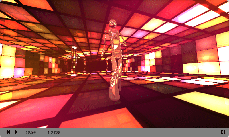
There are a number of ways to implement the effect of fog with modern real time rendered graphics. This blog post will explain how to render fog that has varying density, based on a function of X,Y,Z location in space, like in the picture above.

Faked Fog

One way is to “fake it” and do something like set the color of a pixel on an object to be based on it’s height. For instance you might say that pixels with a y axis value above 15 are unfogged, pixels with y axis values between 15 and 10 progressively get more fogged as they get closer to 10, and pixels with y axis values less than 10 are completely fogged. That can make some fog that looks like this:

heightfog

A strange side effect of doing that though, is if you go down “into” the fog, and look out of the fog, things that should be fogged won’t. For instance, looking up at a mountain from inside the fog, the mountain won’t be fogged at all, even though it should be because you are inside of the fog.

A better way to do it, if you intend for the camera to be able to go into the fog, is to calculate a fogging amount for a pixel based on how far away it is from the view point, and how dense the fog is between the view point and the destination point.

If you are doing ray based rendering, like ray tracing or ray marching, you might find yourself trying to find how much fog is between points that don’t involve the view point – like if you are calculating the reflection portion of a ray. In this case, you are just finding out how much fog there is between the point where the reflection happened and the closest intersection. You can consider the point of reflection as the “view point” for the purpose of fogging.

Sometimes, the entire scene might not be in fog. In this case, you have to find where the fog begins and ends, instead of the total distance between the view point and the destination point.

In any case, the first thing you need to do when fogging is figure out the point where the fog begins, and the point where the fog ends. Then, you can figure out how much fog there is based on how the fog density works.

Constant Density Fog

GraphConstant

The simplest sort of fog is fog that has the same density all throughout it.

What you do in this case is just multiply the fog density by the distance spent in the fog to come up with a final fog value.

As an example, your fog density might be “0.04” and if you are fogging a pixel 10 units away, you multiply density by distance. FogAmount = 0.04 * 10.0 = 0.4.

Doing this, you know the pixel should be 40% fogged, so you interpolate the pixel’s color 40% towards the fog color. You should make sure to clamp the fog amount to be between 0 and 1 to avoid strange visual anomolies.

The image below shows a constant fog density of 0.04.

ConstantFog1

Here’s an image of the same constant density fog as viewed from inside the fog:

ConstantFog3

A problem with constant fog density though, is that if you view it from edge on, you’ll get a very noticeable hard edge where the fog begins, like you can see in the image below:

ConstantFog2

Linear Density Fog

GraphLinear

With linear fog density, the fog gets denser linearly, the farther you go into the fog.

With a fog plane, you can get the density of the fog for a specified point by doing a standard “distance from plane to point” calculation and multiplying that by how much the fog density grows per unit of distance. If your plane is defined by A*x+B*y+C*y+D = 0, and your point is defined as X,Y,Z, you just do a dot product between the plane and the point, giving the point a W component of one.

In other words…

FogDensity(Point, Plane) = (Plane.NormX * Point.X + Plane.NormY * Point.Y + Plane.NormZ * Point.Z + Plane.D * 1.0) * FogGrowthFactor

Here’s a picture of linear fog with a fog growth factor of 0.01:

LinearFog1

The same fog viewed from the inside:

LinearFog2

And lastly, the fog viewed edge on to show that the “hard line” problem of linear fog is gone (dramatic difference isn’t it?!):

LinearFog3

Analytic Fog Density – Integrals

GraphAnalytic

Taking a couple steps further, you might want to use equations to define fog density with some function FogDensity = f(x,y,z,).

How could you possibly figure out how much fog there is between two given points when the density between them varies based on some random function?

One way would be to take multiple samples along the line segment between the view point and the destination point, and either calculate the fog amount in each section, or maybe average the densities you calculate and multiply the result by the total distance. You might have to take a lot of samples to make this look correct, causing low frame rate, or accepting low visual quality as a compromise.

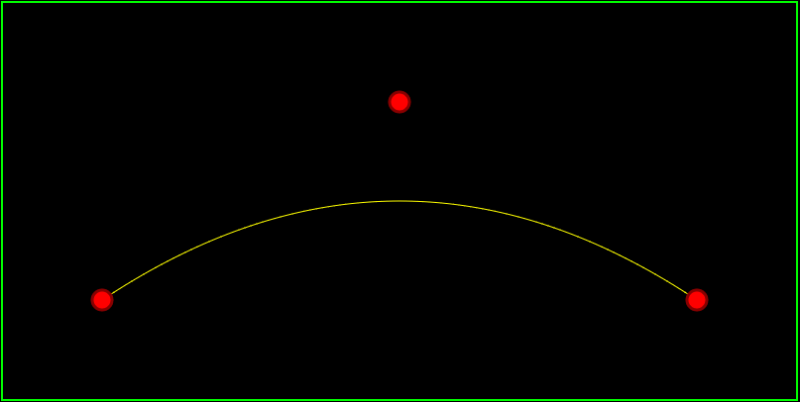
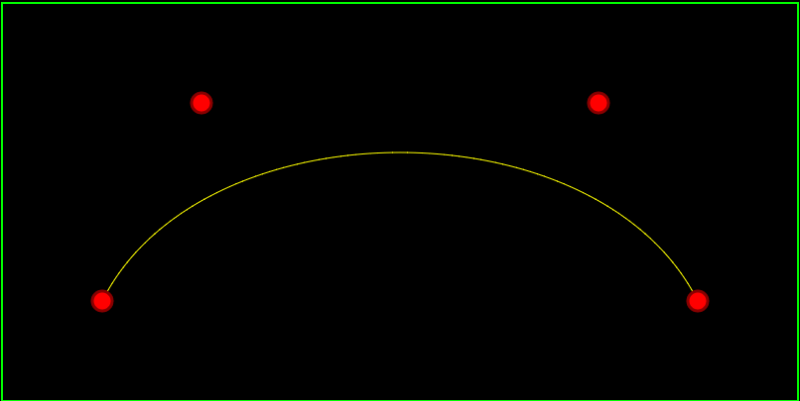
If you look at the graphs for the previous fog types, you might notice that we are trying to find the area under the graphs between points A and B. For constant density fog, the shape is a rectangle, so we just multiply width (time in fog) by height (the constant fog density) to get the fog amount. For linear density fog, the shape is a trapezoid, so we use the trapezoid area formula which is height (in this case, the distance in the fog) times the sum of the base lengths (the fog densities at points A and B) divided by 2.

How can we get the area under the graph between A and B for an arbitrary formula though? Well, a way exists luckily, using integrals (thanks to my buddy “Danny The Physicist” for educating me on the basics of integrals!).

There’s a way to transform a formula to get an “indefinite integral”, which itself is also a formula. I won’t go into the details of how to do that, but you can easily get the indefinite integral of a function by typing it into Wolfram Alpha.

Once you have the indefinite integral (let’s call it G(x)) of the fog density formula (let’s call it F(x)), if you calculate G(B) – G(A), that will give you the area under the graph in F(X) between A and B. Yes, seriously, that gives us the area under the graph between our points, thus giving us the amount of fog that exists between the two points for an arbitrary fog density function!

Note that when you plug a value into the indefinite integral and get a number out, that number is called the definite integral.

Analytic Fog Density – Implementation Details

Now that the theory is worked out let’s talk about implementation details.

First off, coming from an additive audio synthesis type of angle, I figured I might have some good luck adding together sine waves of various frequencies and amplitudes, so I started with this:

sin(x*F) * A

F is a frequency multiplier that controls how long the sine wave is. A is an amplitude multiplier that controls how dense the fog gets max.

Next, I knew that I needed a fog density function that never goes below zero, because that would mean if you looked through a patch of negative fog density, it would make the other fog you were looking through be less dense. That is just weird, and doesn’t exist in reality (but maybe there is some interesting visual effect hiding in there somewhere??), so the formula evolved to this, making sure the function never went below zero:

(1 + sin(x*F)) * A

Plugging that equation into wolfram alpha, it says the indefinite integral is:

(x – (cos(x*F)) / F) * A

You can check that out here:
Wolfram Alpha: (1 + sin(x*F)) * A.

It’s also kind of fun to ask google to graph these functions so you can see what they do to help understand how they work. Here are the graphs for A = 0.01 and F = 0.6:
Fog Density: graph (1 + sin(x*0.6)) * 0.01
Indefinite Integral: graph (x – (cos(x*0.6)) / 0.6) * 0.01

So, if you have point A and B where the fogging begins and ends, you might think you can do this to get the right answer:
FogAmount = G(B.x) – G(A.x)

Nope! There’s a catch. That would work if A and B had no difference on the y or z axis, but since they probably do, you need to jump through some hoops. In essence, you need to stretch your answer across the entire length of the line segment between A and B.

To do that, firstly you need to get that fog amount down to unit length. You do that by modifying the formula like so:
FogAmount = (G(B.x) – G(A.x)) / (B.x – A.x)

This also has a secondary benefit of making it so that your fog amount is always positive (so long as your fog density formula F(X) can’t ever go negative!), which saves an abs() call. Making it always positive ensures that this works when viewing fog both from the left and the right.

Now that we have the fog amount down to unit length, we need to scale it to be the length of the line segment, which makes the formula into this:
FogAmount = (G(B.x) – G(A.x)) * Length(B-A)/(B.x – A.x)

That formula will now give you the correct fog amount.

But, one axis of fog wasn’t enough to look very good, so I wanted to make sure and do one sine wave on each axis. I used 0.01 amplitude for each axis, but for the X axis i used a frequency of 0.6, for the Y axis i used a frequency of 1.2 and for the Z axis i used a frequency of 0.9.

Also, I wanted to give a little bit of baseline fog, so I added some constant density fog in as well, with a constant density of 0.1.

As a bonus, I also gave each axis a “movement factor” that made the sine waves move over time. X axis had a factor of 2.0, Y axis had a factor of 1.4 and Z axis had a factor of 2.2.

Putting all of this together, here is the final fog equation (GLSL pixel shader code) for finding the fog amount between any two points at a specific point in time:

//=======================================================================================
float DefiniteIntegral (in float x, in float amplitude, in float frequency, in float motionFactor)
{
	// Fog density on an axis:
	// (1 + sin(x*F)) * A
	//
	// indefinite integral:
	// (x - cos(F * x)/F) * A
	//
	// ... plus a constant (but when subtracting, the constant disappears)
	//
	x += iGlobalTime * motionFactor;
	return (x - cos(frequency * x)/ frequency) * amplitude;
}

//=======================================================================================
float AreaUnderCurveUnitLength (in float a, in float b, in float amplitude, in float frequency, in float motionFactor)
{
	// we calculate the definite integral at a and b and get the area under the curve
	// but we are only doing it on one axis, so the "width" of our area bounding shape is
	// not correct.  So, we divide it by the length from a to b so that the area is as
	// if the length is 1 (normalized... also this has the effect of making sure it's positive
	// so it works from left OR right viewing).  The caller can then multiply the shape
	// by the actual length of the ray in the fog to "stretch" it across the ray like it
	// really is.
	return (DefiniteIntegral(a, amplitude, frequency, motionFactor) - DefiniteIntegral(b, amplitude, frequency, motionFactor)) / (a - b);
}

//=======================================================================================
float FogAmount (in vec3 src, in vec3 dest)
{
	float len = length(dest - src);
	
	// calculate base fog amount (constant density over distance)	
	float amount = len * 0.1;
	
	// calculate definite integrals across axes to get moving fog adjustments
	float adjust = 0.0;
	adjust += AreaUnderCurveUnitLength(dest.x, src.x, 0.01, 0.6, 2.0);
	adjust += AreaUnderCurveUnitLength(dest.y, src.y, 0.01, 1.2, 1.4);
	adjust += AreaUnderCurveUnitLength(dest.z, src.z, 0.01, 0.9, 2.2);
	adjust *= len;
	
	// make sure and not go over 1 for fog amount!
	return min(amount+adjust, 1.0);
}

More Info

I ended up only using one sine wave per axis, but I think with more sine waves, or perhaps different functions entirely, you could get some more convincing looking fog.

At some point in the future, I’d like to play around with exponential fog density (instead of linear) where the exponential power is a parameter.

I also think that maybe squaring the sine waves could make them have sharper density changes perhaps…

One thing that bugs me in the above screenshots is the obvious “hard line” in both constant and linear fog where it seems fog crosses a threshold and gets a lot denser. I’m not really sure how to fix that yet. In traditional rasterized graphics you could put the fog amount on a curve, to give it a smoother transition, but in ray based rendering, that could make things a bit odd – like you could end up with an exponential curve butting up against the start of a different exponential curve (due to reflection or refraction or similar). The fog density would end up looking like log graph paper which would probably not look so great – although honestly I haven’t tried it to see yet!

If you have any questions, or feedback about improvements you know about or have discovered in any of the above, post a comment and let me know!

Here’s a good read on fog defined by a plane, that also gets into how to make branchless calculations for the fog amounts.
Unified Distance Formulas for Halfspace Fog

Interactive ShaderToy.com demo with GLSL pixel shader source code that you can also edit in real time with WebGL:
Fog

Bezier Curves Part 2 (and Bezier Surfaces)

This is a follow up post to Bezier Curves. My plan was to write a post about b-splines and nurbs next, but after looking into them deeper, I found out they aren’t going to work for my needs so I’m scratching that.

Here’s some basic info on b-splines and nurbs though before diving deeper into Bezier curves and surfaces.

B-Splines (Basis Splines)

Bezier curves are nice, but the more control points you add, the more complex the math gets because the degree of the curve function increases with each control point added. You can put multiple Bezier curves end to end to be able to have more intricate curves, but another option is to use B-Splines.

B-Splines are basically Bezier curves which let you specify more control points without raising the degree of the Bezier curve. They do this by having control points only affect part of the total curve.

This way, you could make a quadratic b-spline which had 10 control points. Only a few control points control any given point on the curve, so the curve stays quadratic (and so does the math), but you get a lot more control points. A “Knot Vector” is what controls which parts of the curve the control points control.

A Bezier curve is actually a special case of B-Spline where all control points affect the entire curve.

Nurbs (Non Uniform Rational B-Spline)

Sometimes when working with curves, you want some control points to be stronger that others. You can accomplish this in Bezier curves and B-splines by doubling up or trippling up control points in the same location to make that control point twice, or three times as strong respectively.

What if you want a control point to be 1.3 times stronger though? That gets a lot more complicated.

Nurbs solve that problem by letting you specify a weight per control point.

Just like Bezier curves are a special case of B-Splines, B-Splines are a special case of nurbs. A B-Spline could be thought of as nurbs that has the same weighting for all control points.

Back to Bezier!

My end goal is to find a curve / surface type that is flexible enough to be used to make a variety of shapes by artists, but is efficient at doing line segment tests against on the GPU. To this end, B-Splines and Nurbs add algorithmic and mathematical complexity over Bezier curves, and seem to be out of the running unless I can’t find anything more promising.

My best bet right now looks like a Bezier Triangle. Specifically, a quadratic Bezier triangle, where each side of the triangle is a quadratic Bezier curve that has 3 control points. When I get those details fully worked out, I’ll report back, but for now, here’s some interesting info I found about generalizing bezier curves both in order (linear, quadratic, cubic, quartic, etc) as well as in the number of dimensions (line, curve, triangle, tetrahedron, etc).

Bezier Generalized

I found the generalized equation on the wikipedia page for Bezier triangles and am super glad i found it, it is very cool!

I want to show you some specifics to explain the generalization by example.

Quadratic Curve:
(A * S + B * T) ^ 2

Expanding that gives you:
A^2 * S^2 + A * B * 2 * S * T + B^2 * T^2

In the above, S and T are Barycentric Coordinates in a 1 dimensional Simplex. Since we know that barycentric coordinates always add up to 1, we can replace S with (1-T) to get the below:

A^2 * (1-T)^2 + A * B * 2 * (1-T) * T + B^2 * T^2

Now, ignoring T and the constants, and only looking at A and B, we have 3 forms: A^2, AB and B^2. Those are our 3 control points! Let’s replace them with A,B and C to get the below:

A * (1-T)^2 + B * 2 * (1-T) * T + C * T ^2

And there we go, there’s the quadratic Bezier curve formula seen in the previous post.

Cubic Curve:
(A * S + B * T) ^ 3

To make a cubic curve, you just change the power from 2 to 3, that’s all! If you expand that equation, you get:
A^3*S^3+3*A^2*B*S^2*T+3*A*B^2*S*T^2+B^3*T^3

We can swap S with (1-T) to get:

A^3*(1-T)^3+3*A^2*B*(1-T)^2*T+3*A*B^2*(1-T)*T^2+B^3*T^3

Looking at A/B terms we see that there is more this time: A^3, A^2B, AB^2 and B^3. Those are our 4 control points that we can replace with A,B,C,D to get:
A*(1-T)^3+3*B*(1-T)^2*T+3*C*(1-T)*T^2+D*T^3

There is the cubic Bezier curve equation from the previous chapter.

Linear Curve:
(A * S + B * T) ^ 1

To expand that, we just throw away the exponent. After we replace S with (1-T) we get:
A * (1-T) + B * T

That is the formula for linear interpolation between 2 points – which you could think of as the 2 control points of the curve.

One more example before we can generalize.

Quadratic Bezier Triangle:
(A * S + B * T + C * U) ^ 2

If you expand that you get this:
A^2*S^2+2*A*B*S*T+2*A*C*S*U+B^2*T^2+2*B*C*T*U+C^2*U^2

Looking at combinations of A,B & C you have: A^2, AB, AC, B^2, BC, C^2. Once again, these are your control points, and their names tell you where they lie on the triangle. A Bezier triangle is a triangle where the 3 sides of the triangle are bezier curves. A quadratic bezier triangle has quadratic bezier curves for it’s edges which mean that each side has 3 control points. Those 3 control points are made up of the 3 corners of the triangle, and then 3 more control points, each one being between end points. A^2, B^2 and C^2 represent the 3 corners of the triangle. AB is the third control point for the bezier curve on the edge AB. BC and AC follow that pattern as well! Super easy to remember.

In a cubic Bezier triangle, you get a lot more control points, but a new class of control point too: ABC. This control point is in the middle of the triangle like the name would imply.

Anyways, in the expanded quadratic bezier triangle equation above, when you replace the control points with A,B,C for the triangle corner control points (the squares) and D,E,F for the inbetween control points, you get the bezier triangle equation below:

A*S^2+2*D*S*T+2*E*S*U+B*T^2+2*F*T*U+C*U^2

Note that we are dealing with a simplex in 3d now, so once again, instead of needing ALL Barycentric coordinates (S,T,U) we could pick one and replace it. For instance, we could replace U with (1-S-T) to have one less variable floating around.

All Done for Now

You can use this pattern to expand either in “surface dimension”, or in the dimension of adding more control points (and increasing the order of the equation). I love it because it’s super simple to remember that simple equation, and then just re-calculate the equation you need for whatever your specific usage case is.

If this stuff is confusing, check out the wiki page for Bezier Triangles, it has a great graphic that really shows you what I’m trying to explain:
Bezier Triangle

Next up I either want to make an HTML5 interactive app for messing around with Bezier triangles, or if I can figure out how to intersect a line segment with a quadratic Bezier triangle, i’ll probably just have some real cool looking screenshots to post along w/ the equation I ended up using (;

Special thanks to wolfram alpha for crunching some of these equations. Check it out, it’s really cool!
Wolfram Alpha – Cubic Bezier Curve Expansion

For more bezier fun check out my next Bezier post: One Dimensional Bezier Curves.

Bezier Curves

Bezier curves are pretty cool. They were invented in the 1950s by Pierre Bezier while he was working at the car company Renault. He created them as a succinct way of describing curves mathematically that could be shared easily with other people, or programmed into machines to make curves that matched the ones created by human designers.

I’m only going to go over bezier curves at the very high level, and give some links to html5 demos I’ve made to let you play around with them and understand how they work, so you too can implement them easily in your own software.

If you want more detailed information, I strongly recommend this book: Focus on Curves and Surfaces

Quadratic Bezier Curves

Quadratic bezier curves have 3 control points. The first control point is where the curve begins, the second control point is a true control point to influence the curve, and the third control point is where the curve ends. Click the image below to be taken to my quadratic bezier curve demo.


bezquad

A quadratic bezier curve has the following parameters:

  • t – the “time” parameter, this parameter goes from 0 to 1 to get the points of the curve.
  • A – the first control point, which is also where the curve begins.
  • B – the second control point.
  • C – the third control point, which is also where the curve ends.

To calculate a point on the curve given those parameters, you just sum up the result of these 3 functions:

  1. A * (1-t)^2
  2. B * 2t(1-t)
  3. C * t^2

In otherwords, the equation looks like this:

CurvePoint = A*(1-t)^2 + B*2t(1-t) + C*t^2

To make an entire curve, you would start with t=0 to get the starting point, t=1 to get the end point, and a bunch of values in between to get the points on the curve itself.

Cubic Bezier Curves

Cubic bezier curves have 4 control points. The first control point is where the curve begins, the second and third control points are true control point to influence the curve, and the fourth control point is where the curve ends. Click the image below to be taken to my cubic bezier curve demo.


bezcubic

A cubic bezier curve has the following parameters:

  • t – the “time” parameter, this parameter goes from 0 to 1 to get the points of the curve.
  • A – the first control point, which is also where the curve begins.
  • B – the second control point.
  • C – the second control point.
  • D – the fourth control point, which is also where the curve ends.

To calculate a point on the curve given those parameters, you just sum up the result of these 4 functions:

  1. A * (1-t)^3
  2. B * 3t(1-t)^2
  3. C * 3t^2(1-t)
  4. D * t^3

In otherwords, the equation looks like this:

CurvePoint = A*(1-t)^3 + B*3t(1-t)^2 + C*3t^2(1-t) + D*t^3

Math

You might think the math behind these curves has to be pretty complex and non intuitive but that is not the case at all – seriously! The curves are based entirely on linear interpolation.

Here are 2 ways you may have seen linear interpolation before.

  1. value = min + percent * (max – min)
  2. value = percent * max + (1 – percent) * min

We are going to use the 2nd form and replace “percent” with “t” but they have the same meaning.

Ok so considering quadratic bezier curves, we have 3 control points: A, B and C.

The formula for linearly interpolating between point A and B is this:
point = t * B + (1-t) * A

The formula for linearly interpolating between point B and C is this:
point = t * C + (1-t) * B

Now, here’s where the magic comes in. What’s the formula for interpolating between the AB formula and the BC formulas above? Well, let’s use the AB formula as min, and the BC formula as max. If you plug the formulas into the linear interpolation formula you get this:

point = t * (t * C + (1-t) * B) + (1-t) * (t * B + (1-t) * A)

if you expand that and simplify it you will end up with this equation:
point = A*(1-t)^2 + B*2t(1-t) + C*t^2

which as you may remember is the formula for a quadratic bezier curve. There you have it… a quadratic bezier curve is just a linear interpolation between 2 other linear interpolations.

Cubic bezier curves work in a similar way, there is just a 4th point to deal with.

Next Up

The demos above are in 2d, but you could easily move to 3d (or higher dimensions!) and use the same equations. Also, there are higher order bezier curves (more control points), but as you add control points, the computational complexity increases, so people usually stick to quadratic or cubic bezier curves, and just string them together. When you put curves end to end like that, they call it a spline.

Next up, be on the look out for posts and demos for b-splines and nurbs!

Soft Maximum vs Hard Maximum

The other day i stumbled on an interesting concept called a “Soft Maximum”.

If you think of the normal maximum, you might have something like this:

float maxValue = max(valueA, valueB);

if valueA and valueB come from functions, there’s usually going to be a sharp bend in the graph of the above where the maximum value changes from valueA to valueB or vice versa.

Sometimes, instead of a sharp bend, you would like a smooth transition between the two values – like when using this for graphics or advanced mathematics.

Here’s the formula for soft max:

double SoftMaximum(double x, double y)
{
	double maximum = max(x, y);
	double minimum = min(x, y);
	return maximum + log( 1.0 + exp(minimum - maximum) );
}

Here are 2 really interesting links on computing and using soft max:

Soft Maximum

How to Compute the Soft Maximum

Check out the images below for an example of when you might use this. This is from a shadertoy shader The Popular Shader. The first image is with using normal max, and the second image uses soft max.

softminOFF

softminON

Converting RGB to Grayscale

If you were converting an RGB pixel to grayscale, you might be like me and be tempted to just add the red, green and blue components together and divide by 3 to get the grayscale equivalent of the color.

That’s close, but not quite correct!

Red, green and blue are not equal brightness, so doing a straight average gives you biased results.

There’s a wikipedia page on this topic here, but the equation to use is below:
grayScale = red * 0.3f + green * 0.59f + blue * 0.11f;

Here are some sample images to show you the difference.

Color:
color

Average:
avg

Weighted Average Equation:
good

Why?

You might be wondering “why the heck would i want to convert RGB to grayscale?”

Well… if you render a scene once, convert it to grayscale and shove it into the red channel, then render the scene again slightly offset to the side, convert that to grayscale and shove it into the blue channel, you can get some neat images like the below. Red/Blue 3d glasses required, click the images to view the full size versions (;