Count Min Sketch: A Probabilistic Histogram

Count min sketch is a probabilistic histogram that was invented in 2003 by Graham Cormode and S. Muthukrishnan.

It’s a histogram in that it can store objects (keys) and associated counts.

It’s probabilistic in that it lets you trade space and computation time for accuracy.

The count min sketch is pretty similar to a bloom filter, except that instead of storing a single bit to say whether an object is in the set, the count min sketch allows you to keep a count per object. You can read more about bloom filters here: Estimating Set Membership With a Bloom Filter.

It’s called a “sketch” because it’s a smaller summarization of a larger data set.

Inserting an Item

The count min sketch is just a 2 dimensional array, with size of W x D. The actual data type in the array depends on how much storage space you want. It could be an unsigned char, it could be 4 bits, or it could be a uint64 (or larger!).

Each row (value of D) uses a different hash function to map objects to an index of W.

To insert an object, for each row you hash the object using that row’s hash function to get the W index for that object, then increment the count at that position.

In this blog post, I’m only going to be talking about being able to add items to the count min sketch. There are different rules / probabilities / etc for count min sketches that can have objects removed, but you can check out the links at the bottom of this post for more information about that!

Getting an Item Count

When you want to get the count of how many times an item has been added to the count min sketch, you do a similar operation as when you insert.

For each row, you hash the object being asked about with that row’s hash function to get the W index and then get the value for that row at the W index.

This will give you D values and you just return the smallest one.

The reason for this, is because due to hash collisions of various hash functions, your count in a specific slot may have been incorrectly incremented extra times due to other objects hashing to the same object. If you take the minimum value you’ve seen across all rows, you are guaranteed to be taking the value that has the least number of hash collisions, so is guaranteed to be most correct, and in fact guaranteed to be greater than or equal to the actual answer – but never lower than the actual answer.

Dot Product (Inner Product)

If you read the last post on using dot product with histograms to gauge similarity, you might be wondering if you can do a dot product between two count min sketch objects.

Luckily yes, you can! They need to have the same W x D dimensions and they need to use the same hash functions per row, but if that’s true, you can calculate a dot product value very easily.

If you have two count min sketch objects A and B that you want to calculate the dot product for, you dot product each row (D index) of the two count min sketch objects. This will leave you with D dot products and you just return the smallest one. This guarantees that the dot product value you calculate will have the fewest hash collisions (so will be most accurate), and will also guarantee that the estimate is greater that or equal to the actual answer, but will never be lower.

To Normalize Or Not To Normalize

There is a caveat here though with doing a dot product between two count min sketch objects. If you do a normalized dot product (normalize the vectors before doing a dot product, or dividing the answer by the length of the two vectors multiplied together), the guarantee that the dot product is greater than or equal to the true answer no longer holds!

The reason for this is that the formula for doing a normalized dot product is like this:
normalized dot product = dot(A,B) / (length(A)*length(B))

In a count min sketch, the dot(A,B) estimate is guaranteed to greater than or equal to the true value.

The length of a vector is also guaranteed to be greater than or equal to the length of the true vector (the vector made from the actual histogram values).

This means that the numerator and the denominator BOTH have varying levels of overestimation in them. Overestimation in the numerator makes the normalized dot product estimate larger, while overestimation in the denominator makes the normalized dot product estimate smaller.

The result is that a normalized dot product estimate can make no guarantee about being greater than or equal to the true value!

This may or may not be a problem for your situation. Doing a dot product with unnormalized vectors still gives you a value that you can use to compare “similarity values” between histograms, but it has slightly different meaning than a dot product with normalized vectors.

Specifically, if the counts are much larger in one histogram versus another (such as when doing a dot product between multiple large text documents and a small search term string), the “weight” of the larger counts will count for more.

That means if you search for “apple pie”, a 100 page novel that mentions apples 10 times will be a better match than a 1/2 page recipe for apple pie!

When you normalize histograms, it makes it so the counts are “by percentage of the total document length”, which would help our search correctly find that the apple pie recipe is more relevant.

In other situations, you might want to let the higher count weigh stronger even though the occurrences are “less dense” in the document.

It really just depends on what your usage case is.

Calculating W & D

There are two parameters (values) used when calculating the correct W and D dimensions of a count min sketch, for the desired accuracy levels. The parameters are ε (epsilon) and δ (delta).

ε (Epsilon) is “how much error is added to our counts with each item we add to the cm sketch”.

δ (Delta) is “with what probability do we want to allow the count estimate to be outside of our epsilon error rate”

To calculate W and D, you use these formulas:

W = ⌈e/ε⌉
D = ⌈ln (1/δ)⌉

Where ln is “natural log” and e is “euler’s constant”.

Accuracy Guarantees

When querying to get a count for a specific object (also called a “point query”) the accuracy guarantees are:

  1. True Count <= Estimated Count
  2. Estimated Count <= True Count + ε * Number Of Items Added
  3. There is a δ chance that #2 is not true

When doing an unnormalized dot product, the accuracy guarantees are:

  1. True Dot Product <= Estimated Dot Product
  2. Estimated Dot Product <= True Dot Product + ε * Number Of Items Added To A * Number Of Items Added To B
  3. There is a δ chance that #2 is not true

Conservative Update

There is an alternate way to implement adding an item to the cm sketch, which results in provably less error. That technique is called a “Conservative Update”.

When doing a conservative update, you first look at the values in each row that you would normally increment and keep track of the smallest value that you’ve seen. You then only increment the counters that have that smallest value.

The reason this works is because we only look at the smallest value across all rows when doing a look up. So long as the smallest value across all rows increases when you insert an object, you’ve satisfied the requirements to make a look up return a value that is greater than or equal to the true value. The reason this conservative update results in less error is because you are writing to fewer values, which means that there are fewer hash collisions happening.

While this increases accuracy, it comes at the cost of extra logic and processing time needed when doing an update, which may or may not be appropriate for your needs.
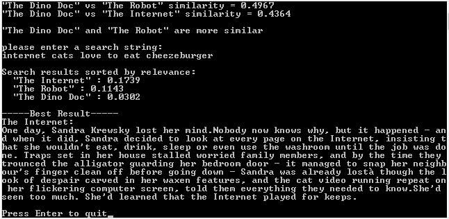
Example Runs

The example program is a lot like the program from the last post which implemented some search engine type functionality.

This program also shows you some count estimations to show you that functionality as well.

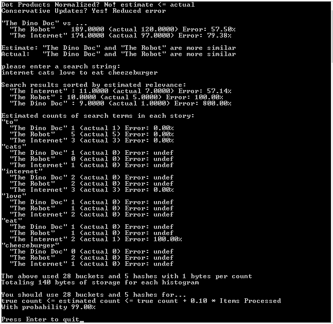
The first run of the program is with normalized vectors, the second run of the program is with unnormalized vectors, and the third run of the program, which is most accurate, is with unnormalized vectors and conservative updates.

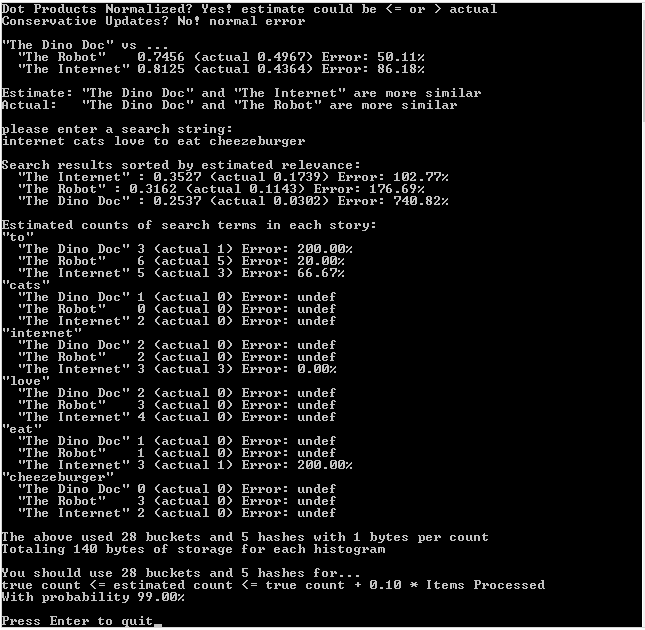
First Run: Normalized Vectors, Regular Updates

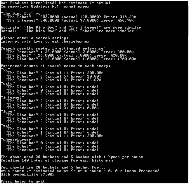
Second Run: Unnormalized Vectors, Regular Updates

Third Run: Unnormalized Vectors, Conservative Updates

Example Code

#include 
#include 
#include 
#include 
#include 
#include 
#include 
#include 

const float c_eulerConstant = (float)std::exp(1.0);

// The CCountMinSketch class
template <typename TKEY, typename TCOUNTTYPE, unsigned int NUMBUCKETS, unsigned int NUMHASHES, typename HASHER = std::hash>
class CCountMinSketch
{
public:
	typedef CCountMinSketch TType;

	CCountMinSketch ()
		: m_countGrid { } // init counts to zero
		, m_vectorLengthsDirty(true)
	{ }

	static const unsigned int c_numBuckets = NUMBUCKETS;
	static const unsigned int c_numHashes = NUMHASHES;
	typedef TCOUNTTYPE TCountType;

	void AddItem (bool conservativeUpdate, const TKEY& item, const TCOUNTTYPE& count)
	{
		// this count min sketch is only supporting positive counts
		if (count = 0!n");
			return;
		}

		// remember that our vector lengths are inaccurate
		m_vectorLengthsDirty = true;

		// if doing a conservative update, only update the buckets that are necesary
		if (conservativeUpdate)
		{
			// find what the lowest valued bucket is and calculate what our new lowest
			// value should be
			TCOUNTTYPE lowestValue = GetCount(item) + count;

			// make sure every bucket has at least the lowest value it should have
			size_t rawHash = HASHER()(item);
			for (unsigned int i = 0; i < NUMHASHES; ++i)
			{
				size_t hash = std::hash()(rawHash ^ std::hash()(i));
				TCOUNTTYPE value = m_countGrid[i][hash%NUMBUCKETS];
				if (value < lowestValue)
					m_countGrid[i][hash%NUMBUCKETS] = lowestValue;
			}
		}
		// else do a normal update
		else
		{
			// for each hash, find what bucket this item belongs in, and add the count to that bucket
			size_t rawHash = HASHER()(item);
			for (unsigned int i = 0; i < NUMHASHES; ++i)
			{
				size_t hash = std::hash()(rawHash ^ std::hash()(i));
				m_countGrid[i][hash%NUMBUCKETS] += count;
			}
		}
	}

	TCOUNTTYPE GetCount (const TKEY& item)
	{
		// for each hash, get the value for this item, and return the smalles value seen
		TCOUNTTYPE ret = 0;
		size_t rawHash = HASHER()(item);
		for (unsigned int i = 0; i < NUMHASHES; ++i)
		{
			size_t hash = std::hash()(rawHash ^ std::hash()(i));
			if (i == 0 || ret > m_countGrid[i][hash%NUMBUCKETS])
				ret = m_countGrid[i][hash%NUMBUCKETS];
		}
		return ret;
	}

	void CalculateVectorLengths ()
	{
		// if our vector lengths were previously calculated, no need to do anything
		if (!m_vectorLengthsDirty)
			return;

		// calculate vector lengths of each hash
		for (unsigned int hash = 0; hash < NUMHASHES; ++hash)
		{
			m_vectorLengths[hash] = 0.0f;
			for (unsigned int bucket = 0; bucket < NUMBUCKETS; ++bucket)
				m_vectorLengths[hash] += (float)m_countGrid[hash][bucket] * (float)m_countGrid[hash][bucket];
			m_vectorLengths[hash] = sqrt(m_vectorLengths[hash]);
		}

		// remember that our vector lengths have been calculated
		m_vectorLengthsDirty = false;
	}

	friend float HistogramDotProduct (TType& A, TType& B, bool normalize)
	{
		// make sure the vector lengths are accurate. No cost if they were previously calculated
		A.CalculateVectorLengths();
		B.CalculateVectorLengths();

		// whatever hash has the smallest dot product is the most correct
		float ret = 0.0f;
		bool foundValidDP = false;
		for (unsigned int hash = 0; hash < NUMHASHES; ++hash)
		{
			// if either vector length is zero, don't consider this dot product a valid result
			// we cant normalize it, and it will be zero anyways
			if (A.m_vectorLengths[hash] == 0.0f || B.m_vectorLengths[hash] == 0.0f)
				continue;

			// calculate dot product of unnormalized vectors
			float dp = 0.0f;
			for (unsigned int bucket = 0; bucket  dp)
			{
				ret = dp;
				foundValidDP = true;
			}
		}
		return ret;
	}

private:
	typedef std::array TBucketList;
	typedef std::array TTable;

	TTable m_countGrid;
	bool m_vectorLengthsDirty;
	std::array m_vectorLengths;
};

// Calculate ideal count min sketch parameters for your needs.
unsigned int CMSIdealNumBuckets (float error)
{
	return (unsigned int)std::ceil((float)(c_eulerConstant / error));
}

unsigned int CMSIdealNumHashes (float probability)
{
	return (unsigned int)std::ceil(log(1.0f / probability));
}

typedef std::string TKeyType;
typedef unsigned char TCountType;

typedef CCountMinSketch THistogramEstimate;
typedef std::unordered_map THistogramActual;

// These one paragraph stories are from http://birdisabsurd.blogspot.com/p/one-paragraph-stories.html

// The Dino Doc : http://birdisabsurd.blogspot.com/2011/11/dino-doc.html (97 words)
const char *g_storyA =
"The Dino Doc:n"
"Everything had gone according to plan, up 'til this moment. His design team "
"had done their job flawlessly, and the machine, still thrumming behind him, "
"a thing of another age, was settled on a bed of prehistoric moss. They'd "
"done it. But now, beyond the protection of the pod and facing an enormous "
"tyrannosaurus rex with dripping jaws, Professor Cho reflected that, had he "
"known of the dinosaur's presence, he wouldn't have left the Chronoculator - "
"and he certainly wouldn't have chosen "Stayin' Alive", by The Beegees, as "
"his dying soundtrack. Curse his MP3 player";

// The Robot: http://birdisabsurd.blogspot.com/2011/12/robot.html (121 words)
const char *g_storyB =
"The Robot:n"
"The engineer watched his robot working, admiring its sense of purpose.It knew "
"what it was, and what it had to do.It was designed to lift crates at one end "
"of the warehouse and take them to the opposite end.It would always do this, "
"never once complaining about its place in the world.It would never have to "
"agonize over its identity, never spend empty nights wondering if it had been "
"justified dropping a promising and soul - fulfilling music career just to "
"collect a bigger paycheck.And, watching his robot, the engineer decided that "
"the next big revolution in the robotics industry would be programming "
"automatons with a capacity for self - doubt.The engineer needed some company.";

// The Internet: http://birdisabsurd.blogspot.com/2011/11/internet.html (127 words)
const char *g_storyC =
"The Internet:n"
"One day, Sandra Krewsky lost her mind.Nobody now knows why, but it happened - "
"and when it did, Sandra decided to look at every page on the Internet, "
"insisting that she wouldn't eat, drink, sleep or even use the washroom until "
"the job was done. Traps set in her house stalled worried family members, and by "
"the time they trounced the alligator guarding her bedroom door - it managed to "
"snap her neighbour's finger clean off before going down - Sandra was already "
"lost… though the look of despair carved in her waxen features, and the cat "
"video running repeat on her flickering computer screen, told them everything "
"they needed to know.She'd seen too much. She'd learned that the Internet "
"played for keeps.";

void WaitForEnter ()
{
	printf("nPress Enter to quit");
	fflush(stdin);
	getchar();
}

template 
void ForEachWord (const std::string &source, L& lambda)
{
	size_t prev = 0;
	size_t next = 0;

	while ((next = source.find_first_of(" ,.-":n", prev)) != std::string::npos)
	{
		if ((next - prev != 0))
		{
			std::string word = source.substr(prev, next - prev);
			std::transform(word.begin(), word.end(), word.begin(), ::tolower);
			lambda(word);
		}
		prev = next + 1;
	}

	if (prev < source.size())
	{
		std::string word = source.substr(prev);
		std::transform(word.begin(), word.end(), word.begin(), ::tolower);
		lambda(word);
	}
}

void PopulateHistogram (THistogramEstimate &histogram, const char *text, bool conservativeUpdate)
{
	ForEachWord(text, [&](const std::string &word) {
		histogram.AddItem(conservativeUpdate, word, 1);
	});
}

void PopulateHistogram (THistogramActual &histogram, const char *text)
{
	ForEachWord(text, [&histogram](const std::string &word) {
		histogram[word]++;
	});
}

float HistogramDotProduct (THistogramActual &A, THistogramActual &B, bool normalize)
{
	// Get all the unique keys from both histograms
	std::set keysUnion;
	std::for_each(A.cbegin(), A.cend(), [&keysUnion](const std::pair& v)
	{
		keysUnion.insert(v.first);
	});
	std::for_each(B.cbegin(), B.cend(), [&keysUnion](const std::pair& v)
	{
		keysUnion.insert(v.first);
	});

	// calculate and return the normalized dot product!
	float dotProduct = 0.0f;
	float lengthA = 0.0f;
	float lengthB = 0.0f;
	std::for_each(keysUnion.cbegin(), keysUnion.cend(),
		[&A, &B, &dotProduct, &lengthA, &lengthB]
		(const TKeyType& key)
		{
			// if the key isn't found in either histogram ignore it, since it will be 0 * x which is
			// always anyhow.  Make sure and keep track of vector length though!
			auto a = A.find(key);
			auto b = B.find(key);

			if (a != A.end())
				lengthA += (float)(*a).second * (float)(*a).second;

			if (b != B.end())
				lengthB += (float)(*b).second * (float)(*b).second;

			if (a == A.end())
				return;

			if (b == B.end())
				return;

			// calculate dot product
			dotProduct += ((float)(*a).second * (float)(*b).second);
		}
	);

	// if we don't need to normalize, return the unnormalized value we have right now
	if (!normalize)
		return dotProduct;

	// normalize if we can
	if (lengthA * lengthB <= 0.0f)
		return 0.0f;

	lengthA = sqrt(lengthA);
	lengthB = sqrt(lengthB);
	return dotProduct / (lengthA * lengthB);
}

template 
const char *CalculateError (const T&estimate, const T&actual)
{
	float error = 100.0f * ((float)estimate - (float)actual) / (float)actual;
	if (std::isnan(error) || std::isinf(error))
		return "undef";
	
	// bad practice to return a static local string, dont do this in production code!
	static char ret[256];
	sprintf(ret, "%0.2f%%", error);
	return ret;
}

int main (int argc, char **argv)
{
	// settings
	const bool c_normalizeDotProducts = false;
	const bool c_conservativeUpdate = true;

	// show settings and implication
	printf("Dot Products Normalized? %sn",
		c_normalizeDotProducts
			? "Yes! estimate could be  actual"
			: "No! estimate <= actual");

	printf("Conservative Updates? %snn",
		c_conservativeUpdate
			? "Yes! Reduced error"
			: "No! normal error");	

	// populate our probabilistic histograms.
	// Allocate memory for the objects so that we don't bust the stack for large histogram sizes!
	std::unique_ptr TheDinoDocEstimate = std::make_unique();
	std::unique_ptr TheRobotEstimate = std::make_unique();
	std::unique_ptr TheInternetEstimate = std::make_unique();
	PopulateHistogram(*TheDinoDocEstimate, g_storyA, c_conservativeUpdate);
	PopulateHistogram(*TheRobotEstimate, g_storyB, c_conservativeUpdate);
	PopulateHistogram(*TheInternetEstimate, g_storyC, c_conservativeUpdate);

	// populate our actual count histograms for comparison
	THistogramActual TheDinoDocActual;
	THistogramActual TheRobotActual;
	THistogramActual TheInternetActual;
	PopulateHistogram(TheDinoDocActual, g_storyA);
	PopulateHistogram(TheRobotActual, g_storyB);
	PopulateHistogram(TheInternetActual, g_storyC);

	// report whether B or C is a closer match for A
	float dpABEstimate = HistogramDotProduct(*TheDinoDocEstimate, *TheRobotEstimate, c_normalizeDotProducts);
	float dpACEstimate = HistogramDotProduct(*TheDinoDocEstimate, *TheInternetEstimate, c_normalizeDotProducts);
	float dpABActual = HistogramDotProduct(TheDinoDocActual, TheRobotActual, c_normalizeDotProducts);
	float dpACActual = HistogramDotProduct(TheDinoDocActual, TheInternetActual, c_normalizeDotProducts);
	printf(""The Dino Doc" vs ...n");
	printf("  "The Robot"    %0.4f (actual %0.4f) Error: %sn", dpABEstimate, dpABActual, CalculateError(dpABEstimate, dpABActual));
	printf("  "The Internet" %0.4f (actual %0.4f) Error: %snn", dpACEstimate, dpACActual, CalculateError(dpACEstimate, dpACActual));
	if (dpABEstimate > dpACEstimate)
		printf("Estimate: "The Dino Doc" and "The Robot" are more similarn");
	else
		printf("Estimate: "The Dino Doc" and "The Internet" are more similarn");
	if (dpABActual > dpACActual)
		printf("Actual:   "The Dino Doc" and "The Robot" are more similarn");
	else
		printf("Actual:   "The Dino Doc" and "The Internet" are more similarn");

	// let the user do a search engine style query for our stories!
	char searchString[1024];
	printf("nplease enter a search string:n");
	searchString[0] = 0;
	scanf("%[^n]", searchString);

	struct SSearchResults
	{
		SSearchResults(const std::string& pageName, float rankingEstimated, float rankingActual)
			: m_pageName(pageName)
			, m_rankingEstimated(rankingEstimated)
			, m_rankingActual(rankingActual)
		{ }

		bool operator  other.m_rankingEstimated;
		}

		std::string m_pageName;
		float       m_rankingEstimated;
		float       m_rankingActual;
	};
	std::vector results;

	// preform our search and gather our results!
	std::unique_ptr searchEstimate = std::make_unique();
	THistogramActual searchActual;
	PopulateHistogram(*searchEstimate, searchString, c_conservativeUpdate);
	PopulateHistogram(searchActual, searchString);
	results.push_back(
		SSearchResults(
			"The Dino Doc",
			HistogramDotProduct(*TheDinoDocEstimate, *searchEstimate, c_normalizeDotProducts),
			HistogramDotProduct(TheDinoDocActual, searchActual, c_normalizeDotProducts)
		)
	);
	results.push_back(
		SSearchResults(
			"The Robot",
			HistogramDotProduct(*TheRobotEstimate, *searchEstimate, c_normalizeDotProducts),
			HistogramDotProduct(TheRobotActual, searchActual, c_normalizeDotProducts)
		)
	);
	results.push_back(
		SSearchResults(
			"The Internet",
			HistogramDotProduct(*TheInternetEstimate, *searchEstimate, c_normalizeDotProducts),
			HistogramDotProduct(TheInternetActual, searchActual, c_normalizeDotProducts)
		)
	);
	std::sort(results.begin(), results.end());

	// show the search results
	printf("nSearch results sorted by estimated relevance:n");
	std::for_each(results.begin(), results.end(), [](const SSearchResults& result) {
		printf("  "%s" : %0.4f (actual %0.4f) Error: %sn",
			result.m_pageName.c_str(),
			result.m_rankingEstimated,
			result.m_rankingActual,
			CalculateError(result.m_rankingEstimated, result.m_rankingActual)
		);
	});

	// show counts of search terms in each story (estimated and actual)
	printf("nEstimated counts of search terms in each story:n");
	std::for_each(searchActual.cbegin(), searchActual.cend(), [&] (const std::pair& v)
	{
		// show key
		printf(""%s"n", v.first.c_str());

		// the dino doc
		TCountType estimate = TheDinoDocEstimate->GetCount(v.first.c_str());
		TCountType actual = 0;
		auto it = TheDinoDocActual.find(v.first.c_str());
		if (it != TheDinoDocActual.end())
			actual = it->second;
		printf("  "The Dino Doc" %u (actual %u) Error: %sn", estimate, actual, CalculateError(estimate, actual));

		// the robot
		estimate = TheRobotEstimate->GetCount(v.first.c_str());
		actual = 0;
		it = TheRobotActual.find(v.first.c_str());
		if (it != TheRobotActual.end())
			actual = it->second;
		printf("  "The Robot"    %u (actual %u) Error: %sn", estimate, actual, CalculateError(estimate, actual));

		// the internet
		estimate = TheInternetEstimate->GetCount(v.first.c_str());
		actual = 0;
		it = TheInternetActual.find(v.first.c_str());
		if (it != TheInternetActual.end())
			actual = it->second;
		printf("  "The Internet" %u (actual %u) Error: %sn", estimate, actual, CalculateError(estimate, actual));
	});

	// show memory use
	printf("nThe above used %u buckets and %u hashes with %u bytes per countn",
		THistogramEstimate::c_numBuckets, THistogramEstimate::c_numHashes, sizeof(THistogramEstimate::TCountType));
	printf("Totaling %u bytes of storage for each histogramnn",
		THistogramEstimate::c_numBuckets * THistogramEstimate::c_numHashes * sizeof(THistogramEstimate::TCountType));
	
	// show a probabilistic suggestion
	float error = 0.1f;
	float probability = 0.01f;
	printf("You should use %u buckets and %u hashes for...n", CMSIdealNumBuckets(error), CMSIdealNumHashes(probability));
	printf("true count <= estimated count <= true count + %0.2f * Items ProcessednWith probability %0.2f%%n", error, (1.0f - probability)*100.0f);
	
	WaitForEnter();
	return 0;
}

Links

If you use this in production code, you should probably use a better quality hash.

The rabbit hole on this stuff goes deeper, so if you want to know more, check out these links!

Wikipedia: Count Min Sketch
Count Min Sketch Full Paper
Count Min Sketch AT&T Research Paper
Another CMS paper
And another, with some more info like range query details

Next up I’ll be writing about hyperloglog, which does the same thing as KMV (K-Minimum Values) but is better at it!

Writing a Basic Search Engine AKA Calculating Similarity of Histograms with Dot Product

I came across this technique while doing some research for the next post and found it so interesting that it seemed to warrant it’s own post.

Histograms and Multisets

Firstly, histogram is just a fancy word for a list of items that have an associated count.

If I were to make a histogram of the contents of my office, I would end up with something like:

  • Books = 20
  • Phone = 1
  • Headphones = 2
  • Sombrero = 1 (thanks to the roaming tequilla cart, but that’s another story…)
  • VideoGames = 15
  • (and so on)

Another term for a histogram is multiset, so if you see that word, just think of it as being the same thing.

Quick Dot Product Refresher

Just to make sure we are on the same page, using dot product to get the angle between two vectors is as follows:

cos(theta) = (A * B) / (||A||*||B||)

Or in coder-eese, if A and B are vectors of any dimension:

cosTheta = dot(A,B) / (length(A)*length(B))

To actually do the “dot” portion, you just multiply the X’s by the X’s, the Y’s by the Y’s, the Z’s by the Z’s etc, and add them all up to get a single scalar value. For a 3d vector it would look like this:

dot(A,B) = A.x*B.x + A.y*B.y + A.z*B.z

The value from the formulas above will tell you how similar the direction of the two vectors are.

If the value is 1, that means they are pointing the exact same way. if the value is 0 that means they are perpendicular. If the value is -1 that means they are pointing the exact opposite way.

Note that you can forgo the division by lengths in that formula, and just look at whether the result is positive, negative, or zero, if that’s enough information for your needs. We’ll be using the full on normalized vector version above in this post today though.

For a deeper refresher on dot product check out this link:
Wikipedia: Dot Product

Histogram Dot Products

Believe it or not, if you treat the counts in a histogram as an N dimensional vector – where N is the number of categories in the histogram – you can use the dot product to gauge similarity between the contents of two histograms by using it to get the angular difference between the vectors!

In the normal usage case, histograms have counts that are >= 0, which ends up meaning that two histogram vectors can only be up to 90 degrees apart. That ends up meaning that the result of the dot product of these normalized vectors is going to be from 0 to 1, where 0 means they have nothing in common, and 1 means they are completely the same.

This is similar to the Jaccard Index mentioned in previous posts, but is different. In fact, this value isn’t even linear (although maybe putting it through acos and dividing by pi/2 may make it suitably linear!), as it represents the cosine of an angle, not a percentage of similarity. It’s still useful though. If you have histogram A and are trying to see if histogram B or C is a closer match to A, you can calculate this value for the A/B pair and the A/C pair. The one with the higher value is the more similar pairing.

Another thing to note about this technique is that order doesn’t matter. If you are trying to compare two multisets where order matters, you are going to have to find a different algorithm or try to pull some shenanigans – such as perhaps weighting the items in the multiset based on the order they were in.

Examples

Let’s say we have two bags of fruit and we want to know how similar the bags are. The bags in this case represent histograms / multisets.

In the first bag, we have 3 apples. In the second bag, we have 2 oranges.


If we have a 2 dimensional vector where the first component is apples and the second component is oranges, we can represent our bags of fruit with these vectors:

Bag1 = [3, 0]
Bag2 = [0, 2]

Now, let’s dot product the vectors:

Dot Product = Bag1.Apples * Bag2.Apples + Bag1.Oranges * Bag2.Oranges
= 3*0 + 0*2
= 0

We would normally divide our answer by the length of the Bag1 vector and then the length of the Bag2 vector, but since it’s zero we know that won’t change the value.

From this, we can see that Bag1 and Bag2 have nothing in common!

What if we added an apple to bag 2 though? let’s do that and try the process again.


Bag1 = [3,0]
Bag2 = [1,2]
Dot Product = Bag1.Apples * Bag2.Apples + Bag1.Oranges * Bag2.Oranges
= 3*1 + 0*2
= 3

Next up, we need to divide the answer by the length of our Bag1 vector which is 3, multiplied the length of our Bag2 vector which is the square root of 5.

Cosine Angle (Similarity Value) = 3 / (3 * sqrt(5))
= ~0.45

Lets add an orange to bag 1. That ought to make it more similar to bag 2, so should increase our similarity value of the two bags. Let’s find out if that’s true.


Bag1 = [3,1]
Bag2 = [1,2]
Dot Product = Bag1.Apples * Bag2.Apples + Bag1.Oranges * Bag2.Oranges
= 3*1 + 1*2
= 5

Next, we need to divide that answer by the length of the bag 1 vector which is the square root of 10, multiplied by the length of the bag 2 vector which is the square root of 5.

Cosine Angle (Similarity Value) = 5 / (sqrt(10) * sqrt(5))
= ~0.71

So yep, adding an orange to bag 1 made the two bags more similar!

Example Code

Here’s a piece of code that uses the dot product technique to be able to gauge the similarity of text. It uses this to compare larger blocks of text, and also uses it to allow you to search the blocks of text like a search engine!

#include 
#include 
#include 
#include 
#include 
 
typedef std::unordered_map THistogram;
 
// These one paragraph stories are from http://birdisabsurd.blogspot.com/p/one-paragraph-stories.html
 
// The Dino Doc : http://birdisabsurd.blogspot.com/2011/11/dino-doc.html
const char *g_storyA =
"The Dino Doc:n"
"Everything had gone according to plan, up 'til this moment. His design team "
"had done their job flawlessly, and the machine, still thrumming behind him, "
"a thing of another age, was settled on a bed of prehistoric moss. They'd "
"done it. But now, beyond the protection of the pod and facing an enormous "
"tyrannosaurus rex with dripping jaws, Professor Cho reflected that, had he "
"known of the dinosaur's presence, he wouldn't have left the Chronoculator - "
"and he certainly wouldn't have chosen "Stayin' Alive", by The Beegees, as "
"his dying soundtrack. Curse his MP3 player";
 
// The Robot: http://birdisabsurd.blogspot.com/2011/12/robot.html
const char *g_storyB =
"The Robot:n"
"The engineer watched his robot working, admiring its sense of purpose.It knew "
"what it was, and what it had to do.It was designed to lift crates at one end "
"of the warehouse and take them to the opposite end.It would always do this, "
"never once complaining about its place in the world.It would never have to "
"agonize over its identity, never spend empty nights wondering if it had been "
"justified dropping a promising and soul - fulfilling music career just to "
"collect a bigger paycheck.And, watching his robot, the engineer decided that "
"the next big revolution in the robotics industry would be programming "
"automatons with a capacity for self - doubt.The engineer needed some company.";
 
// The Internet: http://birdisabsurd.blogspot.com/2011/11/internet.html
const char *g_storyC =
"The Internet:n"
"One day, Sandra Krewsky lost her mind.Nobody now knows why, but it happened - "
"and when it did, Sandra decided to look at every page on the Internet, "
"insisting that she wouldn't eat, drink, sleep or even use the washroom until "
"the job was done. Traps set in her house stalled worried family members, and by "
"the time they trounced the alligator guarding her bedroom door - it managed to "
"snap her neighbour's finger clean off before going down - Sandra was already "
"lost… though the look of despair carved in her waxen features, and the cat "
"video running repeat on her flickering computer screen, told them everything "
"they needed to know.She'd seen too much. She'd learned that the Internet "
"played for keeps.";
 
void WaitForEnter ()
{
    printf("nPress Enter to quit");
    fflush(stdin);
    getchar();
}
 
template 
void ForEachWord (const std::string &source, L& lambda)
{
    size_t prev = 0;
    size_t next = 0;
 
    while ((next = source.find_first_of(" ,.-":n", prev)) != std::string::npos)
    {
        if ((next - prev != 0))
        {
            std::string word = source.substr(prev, next - prev);
            std::transform(word.begin(), word.end(), word.begin(), ::tolower);
            lambda(word);
        }
        prev = next + 1;
    }
 
    if (prev < source.size())
    {
        std::string word = source.substr(prev);
        std::transform(word.begin(), word.end(), word.begin(), ::tolower);
        lambda(word);
    }
}
 
void PopulateHistogram (THistogram &histogram, const char *text)
{
    ForEachWord(text, [&histogram](const std::string &word) {
        histogram[word] ++;
    });
}
 
float HistogramDotProduct (THistogram &A, THistogram &B)
{
    // Get all the unique keys from both histograms
    std::set keysUnion;
    std::for_each(A.cbegin(), A.cend(), [&keysUnion](const std::pair& v)
    {
        keysUnion.insert(v.first);
    });
    std::for_each(B.cbegin(), B.cend(), [&keysUnion](const std::pair& v)
    {
        keysUnion.insert(v.first);
    });
 
    // calculate and return the normalized dot product!
    float dotProduct = 0.0f;
    float lengthA = 0.0f;
    float lengthB = 0.0f;
    std::for_each(keysUnion.cbegin(), keysUnion.cend(),
        [&A, &B, &dotProduct, &lengthA, &lengthB]
        (const std::string& key)
        {
            // if the key isn't found in either histogram ignore it, since it will be 0 * x which is
            // always anyhow.  Make sure and keep track of vector length though!
            auto a = A.find(key);
            auto b = B.find(key);
 
            if (a != A.end())
                lengthA += (float)(*a).second * (float)(*a).second;
 
            if (b != B.end())
                lengthB += (float)(*b).second * (float)(*b).second;
 
            if (a == A.end())
                return;
 
            if (b == B.end())
                return;
 
            // calculate dot product
            dotProduct += ((float)(*a).second * (float)(*b).second);        
        }
    );
 
    // normalize if we can
    if (lengthA * lengthB  dpAC)
        printf(""The Dino Doc" and "The Robot" are more similarn");
    else
        printf(""The Dino Doc" and "The Internet" are more similarn");
 
    // let the user do a search engine style query for our stories!
    char searchString[1024];
    printf("nplease enter a search string:n");
    scanf("%[^n]", searchString);
 
    // preform our search and gather our results!
    THistogram search;
    PopulateHistogram(search, searchString);
 
    struct SSearchResults
    {
        SSearchResults (const std::string& pageName, float ranking, const char* pageContent)
            : m_pageName(pageName)
            , m_ranking(ranking)
            , m_pageContent(pageContent)
        { }
 
        bool operator  other.m_ranking;
        }
 
        std::string m_pageName;
        float       m_ranking;
        const char* m_pageContent;
    };
    std::vector results;
 
    results.push_back(SSearchResults("The Dino Doc", HistogramDotProduct(TheDinoDoc, search), g_storyA));
    results.push_back(SSearchResults("The Robot", HistogramDotProduct(TheRobot, search), g_storyB));
    results.push_back(SSearchResults("The Internet", HistogramDotProduct(TheInternet, search), g_storyC));
    std::sort(results.begin(), results.end());
 
    // show the search results
    printf("nSearch results sorted by relevance:n");
    std::for_each(results.begin(), results.end(), [] (const SSearchResults& result) {
        printf("  "%s" : %0.4fn", result.m_pageName.c_str(), result.m_ranking);
    });
 
    // show the most relevant result
    printf("n-----Best Result-----n%sn",results[0].m_pageContent);
 
    WaitForEnter();
    return 0;
}

Here is an example run of this program:

Improvements

Our “search engine” code does work but is pretty limited. It doesn’t know that “cat” and “Kitty” are basically the same, and also doesn’t know that the words “and”, “the” & “it” are not important.

I’m definitely not an expert in these matters, but to solve the first problem you might try making a “thesaurus” lookup table, where maybe whenever it sees “kitten”, “kitty”, “feline”, it translates it to “cat” before putting it into the histogram. That would make it smarter at realizing all those words mean the same thing.

For the second problem, there is a strange technique called tf–idf that seems to work pretty well, although people haven’t really been able to rigorously figure out why it works so well. Check out the link to it at the bottom of this post.

Besides just using this technique for text comparisons, I’ve read mentions that this histogram dot product technique is used in places like machine vision and object classification.

It is a pretty neat technique 😛

Links

Wikipedia: Cosine Similarity – The common name for this technique
Easy Bar Chart Creator – Used to make the example graphs
Wikipedia: tf-idf – Used to automagically figure out which words in a document are important and which aren’t

Estimating Set Membership With a Bloom Filter

Have you ever found yourself in a situation where you needed to keep track of whether or not you’ve seen an item, but the number of items you have to keep track of is either gigantic or completely unbounded?

This comes up a lot in “massive data” situations (like internet search engines), but it can also come up in games sometimes – like maybe having a monster in an MMO game remember which players have tried to attack it before so it can be hostile when it sees them again.

One solution to the game example could be to keep a list of all players the monster had been attacked by, but that will get huge and eat up a lot of memory and take time to search the list for a specific player.

You might instead decide you only want to keep the last 20 players the monster had been attacked by, but that still uses up a good chunk of memory if you have a lot of different monsters tracking this information for themselves, and 20 may be so low, that the monster will forget people who commonly attack it by the time it sees them again.

Enter The Bloom Filter

There is actually an interesting solution to this problem, using a probabilistic data structure called a bloom filter – and before you ask, no, it has nothing to do with graphics. It was invented by a guy named Burton Howard Bloom in 1970.

A bloom filter basically has M number of bits as storage and K number of hashes.

To illustrate an example, let’s say that we have 10 bits and only 1 hash.

When we insert an item, what we want to do is hash that item and then modulus that has value against 10 to get a pseudo-random (but deterministic) value 0-9. That value is the index of the bit we want to set to true. After we set that bit to true, we can consider that item is inserted into the set.

When we want to ask if an item exists in a given bloom filter, what we do is again hash the item and modulus it against 10 to get the 0-9 value again. If that bit is set to false, we can say that item is NOT in the set with certainty, but if it’s true we can only say it MIGHT be in the set.

If the bit is true, we can’t say that for sure it’s part of the set, because something else may have hashed to the same bit and set it, so we have to consider it a maybe, not a definite yes. In fact, with only 10 bits and 1 hash function, with a good hash function, there is a 10% chance that any item we insert will result in the same bit being set.

To be a little more sure of our “maybe” being a yes, and not a false positive, we can do two things… we can increase the number of bits we use for the set (which will reduce collisions), or we can increase the number of hashes we do (although there comes a point where adding more hashes starts decreasing accuracy again).

If we add a second hash, all that means is that we will do a second hash, get a second 0-9 value, and write a one to that bit AS WELL when we insert an item. When checking if an item exists in a set, we also READ that bit to see if it’s true.

For N hashes, when inserting an item into a bloom filter, you get (up to) N different bits that you need to set to 1.

When checking if an item exists in a bloom filter, you get (up to) N different bits, all of which need to be 1 to consider the item in the set.

There are a few mathematical formulas you can use to figure out how many bits and hashes you would want to use to get a desired reliability that your maybes are in fact yeses, and also there are some formulas for figuring out the probability that your maybe is in fact a yes for any given bloom filter in a runtime state.

Depending on your needs and usage case, you may treat your “maybe” as a “yes” and move on, or you could treat a “maybe” as a time when you need to do a more expensive test (like, a disk read?). In those situations, the “no” is the valuable answer, since it means you can skip the more expensive test.

Estimating Item Count In Bloom Filters

Besides being able to test an item for membership, you can also estimate how many items are in any given bloom filter:

EstimatedCount = -(NumBits * ln(1 – BitsOn / NumBits)) / NumHashes

Where BitsOn is the count of how many bits are set to 1 and ln is natural log.

Set Operations On Bloom Filters

If you have two bloom filters, you can do some interesting set operations on them.

Union

One operation you can do with two bloom filters is union them, which means that if you have a bloom filter A and bloom filter B, you end up with a third bloom filter C that contains all the unique items from both A and B.

Besides being able to test this third bloom filter to see if it contains specific items, you can also ask it for an estimated count of objects it contains, which is useful for helping figure out how similar the sets are.

Essentially, if A estimates having 50 items and B estimates having 50 items, and their union, C, estimates having 51 items, that means that the items in A and B were almost all the same (probably).

How you union two bloom filters is you just do a bitwise OR on every bit in A and B to get the bits for C. Simple and fast to calculate.

Intersection

Another operation you can do with two bloom filters is to calculate their intersection. The intersection of two sets is just the items that the two sets have in common.

Again, besides being able to test this third bloom filter for membership of items, you can also use it to get an estimated count of objects to help figure out how similar the sets are.

Similary to the union, you can reason that if the intersection count is small compared to the counts of the individual bloom filters that went into it, that they were probably not very similar.

There are two ways you can calculate the intersection of two bloom filters.

The first way is to do a bitwise AND on every bit in A and B to get the bits for C. Again, super simple and faster to calculate.

The other way just involves some simple math:

Count(Intersection(A,B)) = (Count(A) + Count(B)) – Count(Union(A,B))

Whichever method is better depends on your needs and your usage case.

Jaccard Index

Just like I talked about in the KMV post two posts ago, you can also calculate an estimated Jaccard Index for two bloom filters, which will give you a value between 0 and 1 that tells you how similar two sets are.

If the Jaccard index is 1, that means the sets are the same and contain all the same items. If the Jaccard index is 0, that means the sets are completely different. If the Jaccard index is 0.5 that means that they have half of their items in common.

To calculate the estimated Jaccard Index, you just use this simple formula:

Jaccard Index = Count(Intersection(A,B)) / Count(Union(A,B))

Estimating False Positive Rate

The more items you insert into a bloom filter the higher the false positive rate gets, until it gets to 100% which means all the bits are set and if you ask if it contains an item, it will never say no.

To combat this, you may want to calculate your error rate at runtime and maybe spit out a warning if the error rate starts getting too high, so that you know you need to adjust the number of bits or number of hashes, or at very least you can alert the user that the reliability of the answers has degraded.

Here is the formula to calculate the false positive rate of a bloom filter at runtime:

ErrorRate = (1 – e^(-NumHashes * NumItems / NumBits))^NumHashes

NumItems is the number of unique items that have been inserted into the bloom filter. If you know that exact value somehow you can use that real value, but in the more likely case, you won’t know the exact value, so you can use the estimated unique item count formula described above to get an estimated unique count.

Managing the Error Rate of False Positives

As I mentioned above, there are formulas to figure out how many bits and how many hashes you need, to store a certain number of items with a specific maximum error rate.

You can work this out in advance by figuring out about how many items you expect to see.

First, you calculate the ideal bit count:

NumBits = – (NumItems * ln(DesiredFalsePositiveProbability)) / (ln(2)^2)

Where NumItems is the number of items you expect to put into the bloom filter, and DesiredFalsePositiveProbability is the error rate you want when the bloom filter has the expected number of items in it. The error rate will be lower until the item count reaches NumItems.

Next, you calculate the ideal number of hashes:

NumHashes = NumBits / NumItems * ln(2)

Then, you just create your bloom filter, using the specified number of bits and hashes.

Example Code

Here is some example bloom filter c++ code with all the bells and whistles. Instead of using multiple hashes, I just grabbed some random numbers and xor them against the hash of each item to make more deterministic but pseudo-random numbers (that’s what a hash does too afterall). If you want to use a bloom filter in a more serious usage case, you may want to actually use multiple hashes, and you probably want to use a better hashing algorithm than std::hash.

#include 
#include 
#include 
#include 
#include 
#include 
#include 
 
// If you get a compile error here, remove the "class" from this enum definition.
// It just means your compiler doesn't support enum classes yet.
enum class EHasItem
{
    e_no,
    e_maybe
};
 
// The CBloomFilter class
template <typename T, unsigned int NUMBYTES, unsigned int NUMHASHES, typename HASHER = std::hash>
class CBloomFilter
{
public:
    // constants
    static const unsigned int c_numHashes = NUMHASHES;
    static const unsigned int c_numBits = NUMBYTES*8;
    static const unsigned int c_numBytes = NUMBYTES;
 
    // friends
    template 
    friend float UnionCountEstimate(const CBloomFilter& left, const CBloomFilter& right);
	template 
	friend float IntersectionCountEstimate (const CBloomFilter& left, const CBloomFilter& right);
 
    // constructor
    CBloomFilter (const std::array& randomSalt)
        : m_storage()              // initialize bits to zero
        , m_randomSalt(randomSalt) // store off the random salt to use for the hashes
    { }
 
    // interface
    void AddItem (const T& item)
    {
        const size_t rawItemHash = HASHER()(item);
        for (unsigned int index = 0; index < c_numHashes; ++index)
        {
            const size_t bitIndex = (rawItemHash ^ m_randomSalt[index])%c_numBits;
            SetBitOn(bitIndex);
        }
    }
 
    EHasItem HasItem (const T& item) const
    {
        const size_t rawItemHash = HASHER()(item);
        for (unsigned int index = 0; index < c_numHashes; ++index)
        {
            const size_t bitIndex = (rawItemHash ^ m_randomSalt[index])%c_numBits;
            if (!IsBitOn(bitIndex))
                return EHasItem::e_no;
        }
        return EHasItem::e_maybe;
    }
 
    // probabilistic interface
    float CountEstimate () const
    {
        // estimates how many items are actually stored in this set, based on how many
        // bits are set to true, how many bits there are total, and how many hashes
        // are done for each item.
        return -((float)c_numBits * std::log(1.0f - ((float)CountBitsOn() / (float)c_numBits))) / (float)c_numHashes;
    }
 
    float FalsePositiveProbability (size_t numItems = -1) const
    {
        // calculates the expected error.  Since this relies on how many items are in
        // the set, you can either pass in the number of items, or use the default
        // argument value, which means to use the estimated item count
        float numItemsf = numItems == -1 ? CountEstimate() : (float)numItems;
        return pow(1.0f - std::exp(-(float)c_numHashes * numItemsf / (float)c_numBits),(float)c_numHashes);
    }
     
private:
 
    inline void SetBitOn (size_t bitIndex)
    {
        const size_t byteIndex = bitIndex / 8;
        const uint8_t byteValue = 1 << (bitIndex%8);
        m_storage[byteIndex] |= byteValue;
    }
 
    inline bool IsBitOn (size_t bitIndex) const
    {
        const size_t byteIndex = bitIndex / 8;
        const uint8_t byteValue = 1 << (bitIndex%8);
        return ((m_storage[byteIndex] & byteValue) != 0);
    }
 
    size_t CountBitsOn () const
    {
        // likely a more efficient way to do this but ::shrug::
        size_t count = 0;
        for (size_t index = 0; index < c_numBits; ++index)
        {
            if (IsBitOn(index))
                ++count;
        }
        return count;
    }
     
    // storage of bits
    std::array m_storage;
 
    // Storage of random salt values
    // It could be neat to use constexpr and __TIME__ to make compile time random numbers.
    // That isn't available til like c++17 or something though sadly.
    const std::array& m_randomSalt;
};
 
// helper functions
template 
float UnionCountEstimate (const CBloomFilter& left, const CBloomFilter& right)
{
    // returns an estimated count of the unique items if both lists were combined
    // example: (1,2,3) union (2,3,4) = (1,2,3,4) which has a union count of 4
    CBloomFilter temp(left.m_randomSalt);
    for (unsigned int index = 0; index < left.c_numBytes; ++index)
        temp.m_storage[index] = left.m_storage[index] | right.m_storage[index];
     
    return temp.CountEstimate();
}
 
template 
float IntersectionCountEstimate (const CBloomFilter& left, const CBloomFilter& right)
{
    // returns an estimated count of the number of unique items that are shared in both sets
    // example: (1,2,3) intersection (2,3,4) = (2,3) which has an intersection count of 2
    CBloomFilter temp(left.m_randomSalt);
    for (unsigned int index = 0; index < left.c_numBytes; ++index)
        temp.m_storage[index] = left.m_storage[index] & right.m_storage[index];
     
    return temp.CountEstimate();
}
 
float IdealBitCount (unsigned int numItemsInserted, float desiredFalsePositiveProbability)
{
    // given how many items you plan to insert, and a target false positive probability at that count, this returns how many bits
    // of flags you should use.
    return (float)-(((float)numItemsInserted*log(desiredFalsePositiveProbability)) / (log(2)*log(2)));
}
 
float IdealHashCount (unsigned int numBits, unsigned int numItemsInserted)
{
    // given how many bits you are using for storage, and how many items you plan to insert, this is the optimal number of hashes to use
    return ((float)numBits / (float)numItemsInserted) * (float)log(2.0f);
}
 
// random numbers from random.org
// https://www.random.org/cgi-bin/randbyte?nbytes=40&format=h
// in 64 bit mode, size_t is 64 bits, not 32.  The random numbers below will be all zero in the upper 32 bits!
static const std::array s_randomSalt =
{
    0x6ff3f8ef,
    0x9b565007,
    0xea709ce4,
    0xf7d5cbc7, 
    0xcb7e38e1,
    0xd54b5323,
    0xbf679080,
    0x7fb78dee,
    0x540c9e8a,
    0x89369800
};
 
// data for adding and testing in our list
static const char *s_dataList1[] =
{
    "hello!",
    "blah!",
    "moo",
    nullptr
};
 
static const char *s_dataList2[] =
{
    "moo",
    "hello!",
    "mooz",
    "kitty",
    "here is a longer string just cause",
    nullptr
};
 
static const char *s_askList[] =
{
    "moo",
    "hello!",
    "unf",
    "boom",
    "kitty",
    "mooz",
    "blah!",
    nullptr
};
 
// driver program
void WaitForEnter ()
{
    printf("nPress Enter to quit");
    fflush(stdin);
    getchar();
}
 
void main(void)
{
    CBloomFilter set1(s_randomSalt);
    CBloomFilter set2(s_randomSalt);
	std::set actualSet1;
	std::set actualSet2;
 
    printf("Creating 2 bloom filter sets with %u bytes of flags (%u bits), and %u hashes.nn", set1.c_numBytes, set1.c_numBits, set1.c_numHashes);
 
	// create data set 1
    unsigned int index = 0;
    while (s_dataList1[index] != nullptr)
    {
        printf("Adding to set 1: "%s"n", s_dataList1[index]);
        set1.AddItem(s_dataList1[index]);
		actualSet1.insert(s_dataList1[index]);
        index++;
    }
 
	// create data set 2
    printf("n");
    index = 0;
    while (s_dataList2[index] != nullptr)
    {
        printf("Adding to set 2: "%s"n", s_dataList2[index]);
        set2.AddItem(s_dataList2[index]);
		actualSet2.insert(s_dataList2[index]);
        index++;
    }
 
	// query each set to see if they think that they contain various items
    printf("n");
    index = 0;
    while (s_askList[index] != nullptr)
    {
        printf("Exists: "%s"? %s & %s (actually %s & %s)n",
            s_askList[index],
            set1.HasItem(s_askList[index]) == EHasItem::e_maybe ? "maybe" : "no",
            set2.HasItem(s_askList[index]) == EHasItem::e_maybe ? "maybe" : "no",
			actualSet1.find(s_askList[index]) != actualSet1.end() ? "yes" : "no",
			actualSet2.find(s_askList[index]) != actualSet2.end() ? "yes" : "no");
        index++;
    }

	// show false positive rates
    printf ("nFalse postive probability = %0.2f%% & %0.2f%%n", set1.FalsePositiveProbability()*100.0f, set2.FalsePositiveProbability()*100.0f);
    printf ("False postive probability at 10 items = %0.2f%%n", set1.FalsePositiveProbability(10)*100.0f);
    printf ("False postive probability at 25 items = %0.2f%%n", set1.FalsePositiveProbability(25)*100.0f);
    printf ("False postive probability at 50 items = %0.2f%%n", set1.FalsePositiveProbability(50)*100.0f);
    printf ("False postive probability at 100 items = %0.2f%%n", set1.FalsePositiveProbability(100)*100.0f);

	// show ideal bit counts and hashes.
    const unsigned int itemsInserted = 10;
    const float desiredFalsePositiveProbability = 0.05f;
    const float idealBitCount = IdealBitCount(itemsInserted, desiredFalsePositiveProbability);
    const float idealHashCount = IdealHashCount((unsigned int)idealBitCount, itemsInserted);
    printf("nFor %u items inserted and a desired false probability of %0.2f%%nYou should use %0.2f bits of storage and %0.2f hashesn",
        itemsInserted, desiredFalsePositiveProbability*100.0f, idealBitCount, idealHashCount);

	// get the actual union
	std::set actualUnion;
	std::for_each(actualSet1.begin(), actualSet1.end(), [&actualUnion] (const std::string& s) {
		actualUnion.insert(s);
	});
	std::for_each(actualSet2.begin(), actualSet2.end(), [&actualUnion] (const std::string& s) {
		actualUnion.insert(s);
	});

	// get the actual intersection
	std::set actualIntersection;
	std::for_each(actualSet1.begin(), actualSet1.end(), [&actualIntersection,&actualSet2] (const std::string& s) {
		if (actualSet2.find(s) != actualSet2.end())
			actualIntersection.insert(s);
	});

	// caclulate actual jaccard index
	float actualJaccardIndex = (float)actualIntersection.size() / (float)actualUnion.size();

	// show the estimated and actual counts, and error of estimations
	printf("nSet1: %0.2f estimated, %u actual.  Error: %0.2f%%n",
		set1.CountEstimate(),
		actualSet1.size(),
		100.0f * ((float)set1.CountEstimate() - (float)actualSet1.size()) / (float)actualSet1.size()
	);
	printf("Set2: %0.2f estimated, %u actual.  Error: %0.2f%%n",
		set2.CountEstimate(),
		actualSet2.size(),
		100.0f * ((float)set2.CountEstimate() - (float)actualSet2.size()) / (float)actualSet2.size()
	);

	float estimatedUnion = UnionCountEstimate(set1, set2);
	float estimatedIntersection = IntersectionCountEstimate(set1, set2);
	float estimatedJaccardIndex = estimatedIntersection / estimatedUnion;
	printf("Union: %0.2f estimated, %u actual.  Error: %0.2f%%n",
		estimatedUnion,
		actualUnion.size(),
		100.0f * (estimatedUnion - (float)actualUnion.size()) / (float)actualUnion.size()
	);
	printf("Intersection: %0.2f estimated, %u actual.  Error: %0.2f%%n",
		estimatedIntersection,
		actualIntersection.size(),
		100.0f * (estimatedIntersection - (float)actualIntersection.size()) / (float)actualIntersection.size()
	);
	printf("Jaccard Index: %0.2f estimated, %0.2f actual.  Error: %0.2f%%n",
		estimatedJaccardIndex,
		actualJaccardIndex,
		100.0f * (estimatedJaccardIndex - actualJaccardIndex) / actualJaccardIndex
	);
 
    WaitForEnter();
}

And here is the output of that program:

In the output, you can see that all the existence checks were correct. All the no’s were actually no’s like they should be, but also, all the maybe’s were actually present, so there were no false positives.

The estimated counts were a little off but were fairly close. The first list was estimated at 2.4 items, when it actually had 3. The second list was estimated at 4.44 items when it actually had 5 items.

It’s reporting a very low false positive rate, which falls in line with the fact that we didn’t see any false positives. The projected false positive rates at 10, 25, 50 and 100 items show us that the set doesn’t have a whole lot more capacity if we want to keep the error rate low.

The union, intersection and jaccard index error rate was pretty low, but the error rate was definitely larger than the false positive rate.

Interestingly, if you look at the part which reports the ideal bit and hash count for 10 items, it says that we should actually use FEWER hashes than we do and a couple less bits. You can actually experiment by changing the number of hashes to 4 and seeing that the error rate goes down. In the example code we are actually using TOO MANY hashes, and it’s hurting our probability rate, for the number of items we plan on inserting.

Interesting Idea

I was chatting with a friend Dave, who said he was using a bloom filter like structure to try and help make sure he didn’t try the same genetic algorithm permutation more than once. An issue with that is that hash collisions could thwart the ability for evolution to happen correctly by incorrectly disallowing a wanted permutation from happening just because it happened to hash to the same value as another permutation already tried. To help this situation, he just biased against permutations found in the data structure, instead of completely blocking them out. Basically, if the permutation was marked as “maybe seen” in the data structure, he’d give it some % chance that it would allow it to happen “again” anyways.

Unfortunately, the idea in general turned out to be impractical. He had about 40 bits of genetic information which is about 1 trillion unique items (2^40).

for being able to store only 1 billion items – which is 1000 times smaller – with 5% false positive rate, that would require about 750MB of storage of bits.

Dropping the requirement to being 25% false positive rate, it still requires 350MB, and to 75% requires 70MB. Even at 99% false positive rate allowed, it requires 2.5MB, and we are still 1000 times too small.

So, for 1 trillion permutations, the size of the bloom filter is unfortunately far too large and he ended up going a different route.

The technique of rolling a random number when you get a maybe is pretty neat though, so wanted to mention it (:

Next Up

We’ve now talked about a probabilistic unique value counter (KMV) that can count the number of unique objects seen.

We then talked about a probabilistic set structure (Bloom Filter) that can keep track of set membership of objects.

How about being able to probabilistically store a list of non unique items?

One way to do this would be to have a count with each item seen instead of only having a bit of whether it’s present or not. When you have a count per item, this is known as a multiset, or the more familiar term: histogram.

If you change a bloom filter to have a count instead of a single bit, that’s called a counting bloom filter and completely works.

There’s a better technique for doing this though called count min sketch. Look for a post soon!

Links

Wikipedia: Bloom Filter
Interactive Bloom Filter Demo

Check this out, it’s a physical implementation of a bloom filter (WAT?!)
Wikipedia: Superimposed code

Estimating Counts of Distinct Values with KMV

A few months ago I saw what I’m about to show you for the first time, and my jaw dropped. I’m hoping to share that experience with you right now, as a I share a quick intro to probabilistic algorithms, starting with KMV, otherwise known as K-Minimum Values, which is a Distinct Value (DV) Sketch, or a DV estimator.

Thanks to Ben Deane for exposure to this really interesting area of computer science.

The Setup

Let’s say that you needed a program to count the number of unique somethings that you’ve encountered. The unique somethings could be unique visitors on a web page, unique logins into a server within a given time period, unique credit card numbers, or anything else that has a way for you to get some unique identifier.

One way to do this would be to keep a list of all the things you’ve encountered before, only inserting a new item if it isn’t already in the list, and then count the items in the list when you want a count of unique items. The obvious downside here is that if the items are large and/or there are a lot of them, your list can get pretty large. In fact, it can take an unbounded amount of memory to store this list, which is no good.

A better solution may be instead of storing the entire item in the list, maybe instead you make a 32 bit hash of the item and then add that hash to a list if it isn’t already in the list, knowing that you have at most 2^32 (4,294,967,296) items in the list. It’s a bounded amount of memory, which is an improvement, but it’s still pretty large. The maximum memory requirement there is 2^32 * 4 which is 17,179,869,184 bytes or 16GB.

You may even do one step better and just decide to have 2^32 bits of storage, and when you encounter a specific 32 bit hash, use that as an index and set that specific bit to 1. You could then count the number of bits set and use that as your answer. That only takes 536,870,912 bytes, or 512MB. A pretty big improvement over 16GB but still pretty big. Also, try counting the number of bits set in a 512MB region of memory. That isn’t the fastest operation around 😛

We made some progress by moving to hashes, which put a maximum size amount of memory required, but that came at the cost of us introducing some error. Hashes can have collisions, and when that occurs in our scenarios above, we have no way of knowing that two items hashing to the same value are not the same item.

Sometimes it’s ok though that we only have an approximate answer, because getting an exact answer may require resources we just don’t have – like infinite memory to hold an infinitely large list, and then infinite computing time to count how many items there are. Also notice that the error rate is tuneable if we want to spend more memory. If we used a 64 bit hash instead of a 32 bit hash, our hash collisions would decrease, and our result would be more accurate, at the cost of more memory used.

The Basic Idea

Let’s try something different, let’s hash every item we see, but only store the lowest valued hash we encounter. We can then use that smallest hash value to estimate how many unique items we saw. That’s not immediately intuitive, so here’s the how and the why…

When we put something into a hash function, what we are doing really is getting a deterministic pseudo random number to represent the item. If we put the same item in, we’ll get the same number out every time, and if we put in a different item, we should get a different number out, even if the second item is really similar to the first item. Interestingly the numbers we get out should have no bearing on the nature of the items we put into the hash. Even if the items we put in are similar, the output should be just as different (on average) as if we put in items that were completely different.

This is one of the properties of a good hash function, that it’s output is (usually) evenly distributed, no matter the nature of the input. What that means is that if we put N items into a hash function, those items are on average going to be evenly spaced in the output of the hash, regardless of how similar or different they were before going into the hash function.

Using this property, the distance from zero to the smallest hash we’ve ever seen can be treated as a representative estimate of the average distance between each item that we hashed. So, to get the number of items in the hash, we convert the smallest hash into a percentage from 0 to 1 of the total hash space (for uint32, convert to float and divide by (float)2^32), and then we can use this formula:

numItems = (1 / percentage) – 1

To understand why we subtract the 1, imagine that our minimum hash value is 0.5. If that is an accurate representation of the space between values, that means that we only have 1 value, right in the middle. But, if we didvide 1 by 0.5 we get 2. We have 2 REGIONS, but we have only 1 item in the list, so we need to subtract 1.

As another example imagine that our minimum hash is 0.3333 and that it is an accurate representation of the space between values. If we divide 1 by 0.3333, we get 3. We do have 3 regions if we cut the whole space into 3 parts, but we only have 2 items (we made 2 cuts to make 3 regions).

Reducing Error

This technique doesn’t suffer too much from hash collisions (so long as your hash function is a decent hash function), but it does have a different sort of problem.

As you might guess, sometimes the hash function might not play nice, and you could hash only a single item, get a hash of 1 and ruin the count estimation. So, there is possibility for error in this technique.

To help reduce error, you ultimately need information about more ranges so that you can combine the multiple pieces of information together to get a more accurate estimate.

Here are some ways to gather information about more ranges:

  • Keep the lowest and highest hash seen instead of just the lowest. This doubles the range information you have since you’d know the range 0-min and max-1.
  • Keep the lowest N hashes seen instead of only the lowest. This multiplies the amount of range information you have by N.
  • Instead of keeping the lowest value from a single hash, perform N hashes instead and keep the lowest value seen from each hash. Again, this multiplies the amount of range information you have by N.
  • Alternately, just salt the same hash N different ways (with high quality random numbers) instead of using N different hash functions, but still keep the lowest seen from each “value channel”. Multiplies info by N again.
  • Also a possibility, instead of doing N hashes or N salts, do a single hash, and xor that hash against N different high quality random numbers to come up with N deterministic pseudorandom numbers per item. Once again, still keep the lowest hash value seen from each “value channel”. Multiplies info by N again
  • Mix the above however you see fit!

Whatever route you go, the ultimate goal is to just get information about more ranges to be able to combine them together.

In vanilla KMV, the second option is used, which is to keep the N lowest hashes seen, instead of just a single lowest hash seen. Thus the full name for KMV: K-Minimum Values.

Combining Info From Multiple Ranges

When you have the info from multiple ranges and need to combine that info, it turns out that using the harmonic mean is the way to go because it’s great at filtering out large values in data that don’t fit with the rest of the data.

Since we are using division to turn the hash value into an estimate (1/percentValue-1), unusually small hashes will result in exponentially larger values, while unusually large hashes will not affect the math as much, but also likely will be thrown out before we ever see them since they will likely not be the minimum hash that we’ve seen.

I don’t have supporting info handy, but from what I’ve been told, the harmonic mean is provably better than both the geometric mean and the regular plain old vanilla average (arithmetic mean) in this situation.

So, to combine information from the multiple ranges you’ve gathered, you turn each range into a distinct value estimate (by calculating 1/percentValue-1) and then putting all those values through the mean equation of your choice (which ought to be harmonic mean, but doesn’t strictly have to be!). The result will be your final answer.

Set Operations

Even though KMV is just a distinct value estimator that estimates a count, there are some interesting probabilistic set operations that you can do with it as well. I’ll be talking about using the k min value technique for gathering information from multiple ranges, but if you use some logic you should be able to figure out how to make it work when you use any of the other techniques.

Jaccard Index

Talking about set operations, I want to start with a concept called the Jaccard index (sometimes called the Jaccard similarity coefficient).

If you have 2 sets, the Jaccard index is calculated by:

Jaccard Index = count(intersection(A,B)) / count(union(A,B))

Since the union of A and B is the combined list of all items in those sets, and the intersection of A and B is the items that they have in common, you can see that if the sets have all items in common, the Jaccard index will be 1 and if the sets have no items in common, the Jaccard index will be 0. If you have some items in common it will be somewhere between 0 and 1. So, the Jaccard Index is just a measurement of how similar two sets are.

Union

If you have the information for two KMV objects, you can get an estimate to the number of unique items there if you were to union them together, even though you don’t have much of the info about the items that are in the set.

To do a union, you just combine the minimum value lists, and remove the K largest ones, so that you are left with the K minimum values from both sets.

You then do business as usual to estimate how many items are in that resulting set.

If you think about it, this makes sense, because if you tracked the items from both lists in a third KMV object, you’d end up with the same K minimums as if you took the K smallest values from both sets individually.

Note that if the two KMV objects are of different size, due to K being different sizes, or because either one isn’t completely filled with K minimum values, you should use the smaller value of K as your union set K size.

Intersection

Finding an estimated count of intersections between two sets is a little bit different.

Basically, having the K minimum hashes seen from both lists, you can think of that as a kind of random sample of a range in both lists. You can then calculate the Jaccard index for that range you have for the two sets (by dividing the size of the intersection by the size of the union), and then use that Jaccard index to estimate an intersection count for the entire set based on the union count estimate.

You can do some algebra to the Jaccard index formula above to get this:

count(intersection(A,B)) = Jaccard Index * count(union(A,B))

Just like with union, if the two KMV objects are of different size, due to K being different sizes, or because either one isn’t completely filled with K minimum values, you should use the smaller value of K.

Sample Code

#include 
#include 
#include 
#include 
#include 
#include 

// The CKMVCounter class
template <typename T, unsigned int NUMHASHES, typename HASHER = std::hash>
class CKMVUniqueCounter
{
public:
	// constants
	static const unsigned int c_numHashes = NUMHASHES;
	static const size_t c_invalidHash = (size_t)-1;

	// constructor
	CKMVUniqueCounter ()
	{
		// fill our minimum hash values with the maximum possible value
		m_minHashes.fill(c_invalidHash);
		m_largestHashIndex = 0;
	}

	// interface
	void AddItem (const T& item)
	{
		// if the new hash isn't smaller than our current largest hash, do nothing
		const size_t newHash = HASHER()(item);
		if (m_minHashes[m_largestHashIndex] <= newHash)
			return;

		// if the new hash is already in the list, don't add it again
		for (unsigned int index = 0; index < c_numHashes; ++index)
		{
			if (m_minHashes[index] == newHash)
				return;
		}

		// otherwise, replace the largest hash
		m_minHashes[m_largestHashIndex] = newHash;

		// and find the new largest hash
		m_largestHashIndex = 0;
		for (unsigned int index = 1; index  m_minHashes[m_largestHashIndex])
				m_largestHashIndex = index;
		}
	}

	// probabilistic interface
	void UniqueCountEstimates (float &arithmeticMeanCount, float &geometricMeanCount, float &harmonicMeanCount)
	{
		// calculate the means of the count estimates.  Note that if there we didn't get enough items
		// to fill our m_minHashes array, we are just ignoring the unfilled entries.  In production
		// code, you would probably just want to return the number of items that were filled since that
		// is likely to be a much better estimate.
		// Also, we need to sort the hashes before calculating uniques so that we can get the ranges by
		// using [i]-[i-1] instead of having to search for the next largest item to subtract out
		SortHashes();
		arithmeticMeanCount = 0.0f;
		geometricMeanCount = 1.0f;
		harmonicMeanCount = 0.0f;
		int numHashes = 0;
		for (unsigned int index = 0; index < c_numHashes; ++index)
		{
			if (m_minHashes[index] == c_invalidHash)
				continue;
			numHashes++;
			float countEstimate = CountEstimate(index);
			arithmeticMeanCount += countEstimate;
			geometricMeanCount *= countEstimate;
			harmonicMeanCount += 1.0f / countEstimate;
		}
		arithmeticMeanCount = arithmeticMeanCount / (float)numHashes;
		geometricMeanCount = pow(geometricMeanCount, 1.0f / (float)numHashes);
		harmonicMeanCount /= (float)numHashes;
		harmonicMeanCount = 1.0f / harmonicMeanCount;
	}

	// friends
	template 
	friend CKMVUniqueCounter KMVUnion (
		const CKMVUniqueCounter& a,
		const CKMVUniqueCounter& b
	);

	template 
	friend float KMVJaccardIndex (
		const CKMVUniqueCounter& a,
		const CKMVUniqueCounter& b
	);

private:

	unsigned int NumHashesSet () const
	{
		unsigned int ret = 0;
		for (unsigned int index = 0; index  0 ? m_minHashes[hashIndex- 1] : 0;
		const float percent = (float)(currentHash-lastHash) / (float)((size_t)-1);
		return (1.0f / percent) - 1.0f;
	}
	
	// the minimum hash values
	std::array m_minHashes;
	size_t m_largestHashIndex;
};

// Set interface
template 
CKMVUniqueCounter KMVUnion (
	const CKMVUniqueCounter& a,
	const CKMVUniqueCounter& b
)
{
	// gather the K smallest hashes seen, where K is the smaller, removing duplicates
	std::set setMinHashes;
	std::for_each(a.m_minHashes.begin(), a.m_minHashes.end(), [&setMinHashes](size_t v) {setMinHashes.insert(v); });
	std::for_each(b.m_minHashes.begin(), b.m_minHashes.end(), [&setMinHashes](size_t v) {setMinHashes.insert(v); });
	std::vector minHashes(setMinHashes.begin(), setMinHashes.end());
	std::sort(minHashes.begin(),minHashes.end());
	minHashes.resize(std::min(a.NumHashesSet(), b.NumHashesSet()));

	// create and return the new KMV union object
	CKMVUniqueCounter ret;
	for (unsigned int index = 0; index < minHashes.size(); ++index)
		ret.m_minHashes[index] = minHashes[index];
	ret.m_largestHashIndex = ret.c_numHashes - 1;
	return ret;
}

template 
float KMVJaccardIndex (
	const CKMVUniqueCounter& a,
	const CKMVUniqueCounter& b
)
{
	size_t smallerK = std::min(a.NumHashesSet(), b.NumHashesSet());

	size_t matches = 0;
	for (size_t ia = 0; ia < smallerK; ++ia)
	{
		for (size_t ib = 0; ib < smallerK; ++ib)
		{
			if (a.m_minHashes[ia] == b.m_minHashes[ib])
			{
				matches++;
				break;
			}
		}
	}

	return (float)matches / (float)smallerK;
}

// data to add to the lists
const char *s_boyNames[] =
{
	"Loki",
	"Alan",
	"Paul",
	"Stripes",
	"Shelby",
	"Ike",
	"Rafael",
	"Sonny",
	"Luciano",
	"Jason",
	"Brent",
	"Jed",
	"Lesley",
	"Randolph",
	"Isreal",
	"Charley",
	"Valentin",
	"Dewayne",
	"Trent",
	"Abdul",
	"Craig",
	"Andre",
	"Brady",
	"Markus",
	"Randolph",
	"Isreal",
	"Charley",
	"Brenton",
	"Herbert",
	"Rafael",
	"Sonny",
	"Luciano",
	"Joshua",
	"Ramiro",
	"Osvaldo",
	"Monty",
	"Mckinley",
	"Colin",
	"Hyman",
	"Scottie",
	"Tommy",
	"Modesto",
	"Reginald",
	"Lindsay",
	"Alec",
	"Marco",
	"Dee",
	"Randy",
	"Arthur",
	"Hosea",
	"Laverne",
	"Bobbie",
	"Damon",
	"Les",
	"Cleo",
	"Robt",
	"Rick",
	"Alonso",
	"Teodoro",
	"Rodolfo",
	"Ryann",
	"Miki",
	"Astrid",
	"Monty",
	"Mckinley",
	"Colin",
	nullptr
};

const char *s_girlNames[] =
{
	"Chanel",
	"Colleen",
	"Scorch",
	"Grub",
	"Anh",
	"Kenya",
	"Georgeann",
	"Anne",
	"Inge",
	"Georgeann",
	"Anne",
	"Inge",
	"Analisa",
	"Ligia",
	"Chasidy",
	"Marylee",
	"Lashandra",
	"Frida",
	"Katie",
	"Alene",
	"Brunilda",
	"Zoe",
	"Shavon",
	"Anjanette",
	"Daine",
	"Sheron",
	"Hilary",
	"Felicitas",
	"Cristin",
	"Ressie",
	"Tynisha",
	"Annie",
	"Sharilyn",
	"Astrid",
	"Charise",
	"Gregoria",
	"Angelic",
	"Lesley",
	"Mckinley",
	"Lindsay",
	"Shanelle",
	"Karyl",
	"Trudi",
	"Shaniqua",
	"Trinh",
	"Ardell",
	"Doreen",
	"Leanna",
	"Chrystal",
	"Treasa",
	"Dorris",
	"Rosalind",
	"Lenore",
	"Mari",
	"Kasie",
	"Ann",
	"Ryann",
	"Miki",
	"Lasonya",
	"Olimpia",
	"Shelby",
	"Lesley",
	"Mckinley",
	"Lindsay",
	"Dee",
	"Bobbie",
	"Cleo",
	"Leanna",
	"Chrystal",
	"Treasa",
	nullptr
};

// driver program
void WaitForEnter ()
{
	printf("nPress Enter to quit");
	fflush(stdin);
	getchar();
}

void main(void)
{
	// how many min values all these KMV objects keep around
	static const int c_numMinValues = 15;

	printf("Using %u minimum valuesnn", c_numMinValues);

	// =====================  Boy Names  =====================
	// put our data into the KVM counter
	CKMVUniqueCounter boyCounter;
	unsigned int index = 0;
	while (s_boyNames[index] != nullptr)
	{
		boyCounter.AddItem(s_boyNames[index]);
		index++;
	}

	// get our count estimates
	float arithmeticMeanCount, geometricMeanCount, harmonicMeanCount;
	boyCounter.UniqueCountEstimates(arithmeticMeanCount, geometricMeanCount, harmonicMeanCount);

	// get our actual unique count
	std::set actualBoyUniques;
	index = 0;
	while (s_boyNames[index] != nullptr)
	{
		actualBoyUniques.insert(s_boyNames[index]);
		index++;
	}

	// print the results!
	printf("Boy Names:n%u actual uniquesn", actualBoyUniques.size());
	float actualCount = (float)actualBoyUniques.size();
	printf("Estimated counts and percent error:n  Arithmetic Mean: %0.2ft%0.2f%%n"
		"  Geometric Mean : %0.2ft%0.2f%%n  Harmonic Mean  : %0.2ft%0.2f%%n",
		arithmeticMeanCount, 100.0f * (arithmeticMeanCount - actualCount) / actualCount,
		geometricMeanCount, 100.0f * (geometricMeanCount - actualCount) / actualCount,
		harmonicMeanCount, 100.0f * (harmonicMeanCount - actualCount) / actualCount);

	// =====================  Girl Names  =====================
	// put our data into the KVM counter
	CKMVUniqueCounter girlCounter;
	index = 0;
	while (s_girlNames[index] != nullptr)
	{
		girlCounter.AddItem(s_girlNames[index]);
		index++;
	}

	// get our count estimates
	girlCounter.UniqueCountEstimates(arithmeticMeanCount, geometricMeanCount, harmonicMeanCount);

	// get our actual unique count
	std::set actualGirlUniques;
	index = 0;
	while (s_girlNames[index] != nullptr)
	{
		actualGirlUniques.insert(s_girlNames[index]);
		index++;
	}

	// print the results!
	printf("nGirl Names:n%u actual uniquesn", actualGirlUniques.size());
	actualCount = (float)actualGirlUniques.size();
	printf("Estimated counts and percent error:n  Arithmetic Mean: %0.2ft%0.2f%%n"
		"  Geometric Mean : %0.2ft%0.2f%%n  Harmonic Mean  : %0.2ft%0.2f%%n",
		arithmeticMeanCount, 100.0f * (arithmeticMeanCount - actualCount) / actualCount,
		geometricMeanCount, 100.0f * (geometricMeanCount - actualCount) / actualCount,
		harmonicMeanCount, 100.0f * (harmonicMeanCount - actualCount) / actualCount);

	// =====================  Set Operations  =====================

	// make the KMV union and get our count estimates
	CKMVUniqueCounter boyGirlUnion = KMVUnion(boyCounter, girlCounter);
	boyGirlUnion.UniqueCountEstimates(arithmeticMeanCount, geometricMeanCount, harmonicMeanCount);

	// make the actual union
	std::set actualBoyGirlUnion;
	std::for_each(actualBoyUniques.begin(), actualBoyUniques.end(),
		[&actualBoyGirlUnion](const std::string& s)
		{
			actualBoyGirlUnion.insert(s);
		}
	);
	std::for_each(actualGirlUniques.begin(), actualGirlUniques.end(),
		[&actualBoyGirlUnion](const std::string& s)
		{
			actualBoyGirlUnion.insert(s);
		}
	);

	// print the results!
	printf("nUnion:n%u actual uniques in unionn", actualBoyGirlUnion.size());
	actualCount = (float)actualBoyGirlUnion.size();
	printf("Estimated counts and percent error:n  Arithmetic Mean: %0.2ft%0.2f%%n"
		"  Geometric Mean : %0.2ft%0.2f%%n  Harmonic Mean  : %0.2ft%0.2f%%n",
		arithmeticMeanCount, 100.0f * (arithmeticMeanCount - actualCount) / actualCount,
		geometricMeanCount, 100.0f * (geometricMeanCount - actualCount) / actualCount,
		harmonicMeanCount, 100.0f * (harmonicMeanCount - actualCount) / actualCount);

	// calculate estimated jaccard index
	float estimatedJaccardIndex = KMVJaccardIndex(boyCounter, girlCounter);

	// calculate actual jaccard index and actual intersection
	size_t actualIntersection = 0;
	std::for_each(actualBoyUniques.begin(), actualBoyUniques.end(),
		[&actualGirlUniques, &actualIntersection] (const std::string &s)
		{
			if (actualGirlUniques.find(s) != actualGirlUniques.end())
				actualIntersection++;
		}
	);
	float actualJaccardIndex = (float)actualIntersection / (float)actualBoyGirlUnion.size();

	// calculate estimated intersection
	float estimatedIntersection = estimatedJaccardIndex * (float)actualBoyGirlUnion.size();

	// print the intersection and jaccard index information
	printf("nIntersection:n%0.2f estimated, %u actual.  Error: %0.2f%%n",
		estimatedIntersection,
		actualIntersection,
		100.0f * (estimatedIntersection - (float)actualIntersection) / (float)actualIntersection);

	printf("nJaccard Index:n%0.2f estimated, %0.2f actual.  Error: %0.2f%%n",
		estimatedJaccardIndex,
		actualJaccardIndex,
		100.0f * (estimatedJaccardIndex-actualJaccardIndex) / actualJaccardIndex
	);

	WaitForEnter();
}

Here’s the output of the program:

Upgrading from Set to Multi Set

Interestingly, if you keep a count of how many times you’ve seen each hash in the k min hash, you can upgrade this algorithm from being a set algorithm to a multi set algorithm and get some other interesting information from it.

Where a set is basically a list of unique items, a multi set is a set of unique items that also have a count associated with them. In this way, you can think of a multiset as just a list of items which may appear more than once.

Upgrading KMV to a multi set algorithm lets you do some new and interesting things where instead of getting information only about unique counts, you can get information about non unique counts too. But to re-iterate, you still keep the ability to get unique information as well, so it is kind of like an upgrade, if you are interested in multiset information.

Links

Want more info about this technique?

Sketch of the Day: K-Minimum Values

Sketch of the Day: Interactive KMV web demo

K-Minimum Values: Sketching Error, Hash Functions, and You

Wikipedia: MinHash – Jaccard similarity and minimum hash values

All Done

I wanted to mention that even though this algorithm is a great, intuitive introduction into probabilistic algorithms, there are actually much better distinct value estimators in use today, such as one called HyperLogLog which seems to be the current winner. Look for a post on HyperLogLog soon 😛

KMV is better than other algorithms at a few things though. Specifically, from what I’ve read, that it can extend to multiset makes it very useful, and also it is much easier to calculate intersections versus other algorithms.

I also wanted to mention that there are interesting usage cases for this type of algorithms in game development, but where these probabilistic algorithms really shine is in massive data situations like google, amazon, netflix etc. If you go out searching for more info on this stuff, you’ll probably be led down many big data / web dev rabbit holes, because that’s where the best information about this stuff resides.

Lastly, I wanted to mention that I’m using the C++ std::hash built in hash function. I haven’t done a lot of research to see how it compares to other hashes, but I’m sure, much like rand(), the built in functionality leaves much to be desired for “power user” situations. In other words, if you are going to use this in a realistic situation, you probably are better off using a better hashing algorithm. If you need a fast one, you might look into the latest murmurhash variant!

More probabilistic algorithm posts coming soon, so keep an eye out!

Programmatically Calculating GCD and LCM

I recently came across a really interesting technique for calculating GCD (greatest common divisor) and then found out you can use that to calculate LCM (least common multiple).

Greatest Common Divisor

The greatest common divisor of two numbers is the largest number that divides evenly into those numbers.

For instance the GCD of 12 and 15 is 3, the GCD of 30 and 20 is 10, and the GCD of 7 and 11 is 1.

You could calculate this with brute force – starting with 1 and counting up to the smaller number, keeping track of the largest number that divides evenly into both numbers – but for larger numbers, this technique could take a long time.

Luckily Euclid came up a better way in 300 BC!

Euclid’s algorithm to find the GCD of numbers A and B:

  1. If A and B are the same number, that number is the GCD
  2. Otherwise, subtract the smaller number from the larger number
  3. Goto 1

Pretty simple right? It’s not immediately intuitive why that works, but as an example let’s say that there’s a number that goes into A fives times, and goes into B three times. That same number must go into (A-B) two times.

Try it out on paper, think about it a bit, and check out the links at the end of this section (:

A refinement on that algorithm is to use remainder (modulus) instead of possibly having to do repeated subtraction to get the same result. For instance if you had the numbers 1015 and 2, you are going to have to subtract 2 from 1015 quite a few times before the 2 becomes the larger number.

Here’s the refined algorithm:

  1. If A and B are the same number, that number is the GCD
  2. Otherwise, set the larger number to be the remainder of the larger number divided by the smaller number
  3. Goto 1

And here’s the C++ code:

#include <stdio.h>
#include <algorithm>

unsigned int CalculateGCD (unsigned int smaller, unsigned int larger)
{
	// make sure A <= B before starting
	if (larger < smaller)
		std::swap(smaller, larger);

	// loop
	while (1)
	{
		// if the remainder of larger / smaller is 0, they are the same
		// so return smaller as the GCD
		unsigned int remainder = larger % smaller;
		if (remainder == 0)
			return smaller;

		// otherwise, the new larger number is the old smaller number, and
		// the new smaller number is the remainder
		larger = smaller;
		smaller = remainder;
	}
}

void WaitForEnter ()
{
	printf("nPress Enter to quit");
	fflush(stdin);
	getchar();
}

void main (void)
{
	// Get A
	printf("Greatest Common Devisor Calculator, using Euclid's algorithm!n");
	printf("nFirst number? ");
	unsigned int A = 0;
	if (scanf("%u",&A) == 0 || A == 0) {
		printf("nMust input a positive integer greater than 0!");
		WaitForEnter();
		return;
	}

	// Get B
	printf("Second number? ");
	unsigned int B = 0;
	if (scanf("%u",&B) == 0 || B == 0) {
		printf("nMust input a positive integer greater than 0!");
		WaitForEnter();
		return;
	}
	
	// show the result
	printf("nGCD(%u,%u) = %un", A, B, CalculateGCD(A,B));

	// wait for user to press enter
	WaitForEnter();
}

I found this stuff in Michael Abrash’s Graphics Programming Black Book Special Edition: Patient Coding, Faster Code.

That book is filled with amazing treasures of knowledge and interesting stories to boot. I highly suggest flipping to a couple random chapters and reading it a bit. Very cool stuff in there (:

You might also find these links interesting or useful!
Wikipedia: Greatest Common Divisor
Wikipedia: Euclidean Algorithm

I’m sure there’s a way to extend this algorithm to work for N numbers at a time instead of only 2 numbers. I’ll leave that as a fun exercise for you if you want to play with that 😛

Least Common Multiple

The least common multiple of two numbers is the smallest number that is evenly divisible by those numbers.

Kind of an ear full so some examples: The LCM of 3 and 4 is 12, the LCM of 1 and 7 is 7, the LCM of 20 and 35 is 140. Note that in the first two examples, the LCM is just the two numbers multiplied together, but in the 3rd example it isn’t (also an interesting thing of note is that the first 2 examples have a GCD of 1, while the 3rd example has a GCD of 5).

Well interestingly, calculating the LCM is super easy if you already know how to calculate the GCD. You just multiply the numbers together and divide by the GCD.

LCM(A,B) = (A*B) / GCD(A,B)

Interestingly though, GCD(A,B) divides evenly into both A and B and will result in an integer result. This means we can multiply by A or B after the division happens and get the exact same answer. More importantly though, it helps protect you against integer overflow in the A*B calculation. Using that knowledge the equation becomes this:

LCM(A,B) = (A / GCD(A,B))*B

Pretty neat! Here’s some C++ code that calculates LCM.

#include <stdio.h>
#include <algorithm>

unsigned int CalculateGCD (unsigned int smaller, unsigned int larger)
{
	// make sure A <= B before starting
	if (larger < smaller)
		std::swap(smaller, larger);

	// loop
	while (1)
	{
		// if the remainder of larger / smaller is 0, they are the same
		// so return smaller as the GCD
		unsigned int remainder = larger % smaller;
		if (remainder == 0)
			return smaller;

		// otherwise, the new larger number is the old smaller number, and
		// the new smaller number is the remainder
		larger = smaller;
		smaller = remainder;
	}
}

unsigned int CalculateLCM (unsigned int A, unsigned int B)
{
	// LCM(A,B) = (A/GCD(A,B))*B
	return (A/CalculateGCD(A,B))*B;
}

void WaitForEnter ()
{
	printf("nPress Enter to quit");
	fflush(stdin);
	getchar();
}

void main (void)
{
	// Get A
	printf("Least Common Multiple Calculator, using Euclid's algorithm for GCD!n");
	printf("nFirst number? ");
	unsigned int A = 0;
	if (scanf("%u",&A) == 0 || A == 0) {
		printf("nMust input a positive integer greater than 0!");
		WaitForEnter();
		return;
	}

	// Get B
	printf("Second number? ");
	unsigned int B = 0;
	if (scanf("%u",&B) == 0 || B == 0) {
		printf("nMust input a positive integer greater than 0!");
		WaitForEnter();
		return;
	}
	
	// show the result
	printf("nLCM(%u,%u) = %un", A, B, CalculateLCM(A,B));

	// wait for user to press enter
	WaitForEnter();
}

Extending this to N numbers could be an interesting thing to try too (:

Here’s tasty link about LCM: Wikipedia: Least Common Multiple

Compile Time GCD and LCM

I’ve just heard that a compile time GCD and LCM implementation has been recomended for the STL. Check out the link below, kinda neat!

Greatest Common Divisor and Least Common Multiple

TTFN.

Bresenham’s Drawing Algorithms

If you were asked to name a line drawing algorithm, chances are you would say Bresenham. I recently needed to write my own software line drawing algorithm (CPU and regular ram, not GPU and VRAM) and Bresenham was the first to come to mind for me as well.

Believe it or not, Jack Bresenham actually came up with 2 famous line drawing algorithms. One is a run length algorithm, and the other is a run slice algorithm. People are most often familiar with the run length algorithm, which I mainly talk about in this post, but there’s some information about the run slice algorithm and links to other Bresenham primitive rendering algorithms below as well!

An interesting thing about both line algorithms is that they involve only integer mathematics, so there is no round off error, epsilons, numerical instability or anything like that. You use only integers and simple math (no divisions even!), and get the exact right answer out. I think that is pretty cool.

Bresenham’s Run Length Line Algorithm Summarized

To help understand the code, I want to give a brief summarization of how the algorithm works at a high level.

The first step of the Bresenham line algorithm is to see if the line is longer on the X axis or Y axis. Whichever one it is longer on is the major axis, and the shorter one is the minor axis.

Then, starting at the starting point of the line, you loop across all pixels of the major axis, doing some math to decide for each pixel whether you need to move the pixel on the minor axis yet or not. Basically you keep track of the error – or the distance the pixel is away from the true position of the line on the minor axis – and if the error is greater than or equal to 1 pixel, you move the pixel on the minor axis and subtract one pixel from the error. If the error is smaller than 1 pixel, you keep it at the same value it was for the last pixel, and keep the error value the same, so that it can accumulate some more error for the next pixel and test again.


The left line is longer on the X axis, so the major axis is the X axis. The right line is longer on the Y axis, so the major axis is the Y axis. Notice that there is one pixel for each value along the major axis of each line, but repeated pixel values along the minor axis of each line.

If you want the deeper details about the algorithm or the math behind it, check out this link:
Wikipedia: Bresenham’s line algorithm

One Octant Code

Wikipedia says that many implementations implement the algorithm for a single octant (half of a quadrant) and then use coordinate conversions (flipping the x and y’s and/or negating them) to make the same logic work for any quadrant.

In that vein, here is a simple implementation for the first octant – where the major axis is X, and both X and Y are increasing from the starting point to the ending point.

	void DrawLine (int x1, int y1, int x2, int y2, unsigned int color)
	{
		const int dx = x2 - x1;
		const int dy = y2 - y1;

		int Error = 2 * dy - dx;
		int y = y1;
		
		DrawPixel(x1, y1, color);
		for (int x = x1+1; x < x2; ++x)
		{
			if (Error > 0)
			{
				y++;
				Error += 2 * dy - 2 * dx;
			}
			else
			{
				Error += 2 * dy;
			}
			DrawPixel(x,y,color);
		}
	}

With the point of Bresenham being that it is efficient, let’s sacrifice readability a bit and get rid of those DrawPixel calls and perhaps over-micro-optimize a bit and make some consts for frequently used values.

	void DrawLine (unsigned int* pixels, int width, int x1, int y1, int x2, int y2, unsigned int color)
	{
		const int dx = x2 - x1;
		const int dy = y2 - y1;
		const int dx2 = dx * 2;
		const int dy2 = dy * 2;
		const int dy2Mindx2 = dy2 - dx2;

		int Error = dy2 - dx;

		unsigned int* pixel = &amp;pixels[y1*width+x1];
		*pixel = color;
		for (int x = x2 - x1 - 1; x > 0; --x)
		{
			if (Error > 0)
			{
				pixel += width + 1;
				Error += dy2Mindx2;
			}
			else
			{
				pixel++;
				Error += dy2;
			}
			*pixel = color;
		}
	}

Cool, now let’s make it work for any line.

Final Code

	// Generic Line Drawing
	// X and Y are flipped for Y maxor axis lines, but the pixel writes are handled correctly due to
	// minor and major axis pixel movement
	void DrawLineMajorAxis(
		unsigned int* pixel,
		int majorAxisPixelMovement,
		int minorAxisPixelMovement,
		int dx,
		int dy,
		unsigned int color
	)
	{
		// calculate some constants
		const int dx2 = dx * 2;
		const int dy2 = dy * 2;
		const int dy2Mindx2 = dy2 - dx2;

		// calculate the starting error value
		int Error = dy2 - dx;

		// draw the first pixel
		*pixel = color;

		// loop across the major axis
		while (dx--)
		{
			// move on major axis and minor axis
			if (Error > 0)
			{
				pixel += majorAxisPixelMovement + minorAxisPixelMovement;
				Error += dy2Mindx2;
			}
			// move on major axis only
			else
			{
				pixel += majorAxisPixelMovement;
				Error += dy2;
			}

			// draw the next pixel
			*pixel = color;
		}
	}

	// Specialized Line Drawing optimized for horizontal or vertical lines
	// X and Y are flipped for Y maxor axis lines, but the pixel writes are handled correctly due to
	// minor and major axis pixel movement
	void DrawLineSingleAxis(unsigned int* pixel, int majorAxisPixelMovement, int dx, unsigned int color)
	{
		// draw the first pixel
		*pixel = color;

		// loop across the major axis and draw the rest of the pixels
		while (dx--)
		{
			pixel += majorAxisPixelMovement;
			*pixel = color;
		};
	}

	// Draw an arbitrary line.  Assumes start and end point are within valid range
	// pixels is a pointer to where the pixels you want to draw to start aka (0,0)
	// pixelStride is the number of unsigned ints to get from one row of pixels to the next.
	// Usually, that is the same as the width of the image you are drawing to, but sometimes is not.
	void DrawLine(unsigned int* pixels, int pixelStride, int x1, int y1, int x2, int y2, unsigned int color)
	{
		// calculate our deltas
		int dx = x2 - x1;
		int dy = y2 - y1;

		// if the X axis is the major axis
		if (abs(dx) >= abs(dy))
		{
			// if x2 < x1, flip the points to have fewer special cases
			if (dx < 0)
			{
				dx *= -1;
				dy *= -1;
				swap(x1, x2);
				swap(y1, y2);
			}

			// get the address of the pixel at (x1,y1)
			unsigned int* startPixel = &amp;pixels[y1 * pixelStride + x1];

			// determine special cases
			if (dy > 0)
				DrawLineMajorAxis(startPixel, 1, pixelStride, dx, dy, color);
			else if (dy < 0)
				DrawLineMajorAxis(startPixel, 1, -pixelStride, dx, -dy, color);
			else
				DrawLineSingleAxis(startPixel, 1, dx, color);
		}
		// else the Y axis is the major axis
		else
		{
			// if y2 < y1, flip the points to have fewer special cases
			if (dy < 0)
			{
				dx *= -1;
				dy *= -1;
				swap(x1, x2);
				swap(y1, y2);
			}

			// get the address of the pixel at (x1,y1)
			unsigned int* startPixel = &amp;pixels[y1 * pixelStride + x1];

			// determine special cases
			if (dx > 0)
				DrawLineMajorAxis(startPixel, pixelStride, 1, dy, dx, color);
			else if (dx < 0)
				DrawLineMajorAxis(startPixel, pixelStride, -1, dy, -dx, color);
			else
				DrawLineSingleAxis(startPixel, pixelStride, dy, color);
		}
	}

Using the above functions, I wrote a little test to draw lines from the center of an image towards the edges at 100 different angles, and also a horizontal and vertical line. Here’s the results:

Run Slice Algorithm

So, like I said above, there is another Bresenham line algorithm that is a run slice algorithm.

What that means is that instead of looping across the major axis figuring out if each pixel needs to move on the minor axis as well, instead it loops across the minor axis, figuring out how many pixels it needs to write for that row or column of pixels.

One benefit of that algorithm is that it is less loop iterations since it’s looping across the minor axis pixels instead of the major axis.

Here’s an interesting read about Michael Abrash and his encounters with and the run slice algorithm:

Michael Abrash’s Graphics Programming Black Book Special Edition: The Good, the Bad, and the Run-Sliced

Other Bresenham Algorithms

This was origionally just going to be about the line algorithms, and I was going to make up another post about the circle algorithm, but I changed my mind.

While doing some research to see if there was a Bresenham bezier curve algorithm I stumbled on the page below, which shows that yes, there is! There are quite a few other algorithms as well:

Many Bresenham algorithms with very short c++ implementations

Dual Numbers & Automatic Differentiation

In the last post, I talked about imaginary numbers, complex numbers, and how to use them to rotate vectors in 2d.

In this post, I want to share another interesting type of number called a “Dual Number” that uses the symbol ε (epsilon) and has a neat trick of automatically calculating the derivative of a function while you calculate the value of the function at the same time.

Dual numbers are pretty similar to imaginary numbers but there is one important difference. With imaginary numbers, i^2 = -1, but with dual numbers, ε^2 = 0 (and ε is not 0!). That may seem like a small difference, but oddly, that opens up a whole interesting world of mathematical usefulness.

Before we dig into automatic differentiation, I want to go over the mathematical basics for how dual numbers behave.

Basic Dual Number Math

Adding dual numbers is the same as adding complex numbers; you just add the real and dual parts separately:

(3 + 4ε) + (1 + 2ε) = 4 + 6ε

Subtraction works the same way as well:

(3 + 4ε) – (1 + 2ε) = 2 + 2ε

To multiply dual numbers, you use F.O.I.L. just like you do with complex numbers:

(3 + 4ε) * (1 + 2ε) =
3 + 6ε + 4ε + 8ε^2 =
3 + 10ε + 8ε^2

However, since ε^2 is zero, the last term 8ε^2 disappears:
3 + 10ε

It’s interesting to note that with complex numbers, the i^2 became -1, so the last term changed from imaginary to real, meaning that the imaginary numbers fed back into the real numbers during multiplication. With dual numbers, that isn’t the case, the dual numbers don’t feed back into the real numbers during multiplication.

In both complex and dual numbers the real terms do affect the non real terms during multiplication.

The division operator relates to the conjugate. I have source code for it below, and some of the links at the end of the post go into the details of that and other operations.

Quick Review: Derivatives (Slope)

If you know the line formula y=mx+b, but you don’t know what a derivative is you are in luck. Remember how “m” is the slope of the line, specifying how steep it is? That is what the derivative is too, it’s just the slope.

Below is a graph of y=2x+1. At every point on that line, the derivative (or slope) is 2. That means that for every step we make on the x axis to the right (positive direction), we make 2 steps up on the y axis (positive direction).

Now, check out this graph of y=x^2-0.2

The derivative (or slope) at every point on this graph is 2x. That means that the slope changes depending on where the x coordinate is!

So, when x=0, the slope is 0. You can see that in the graph where x=0, that it is horizontal, meaning that a step on the x axis becomes no steps on the y axis (only at that point where x is 0, and only if you take an infinitely small step).

When x is 1, the slope is 2, when x is 2, the slope is 4, when x is 3, the slope is 6. Since the numbers increase as we increase x from 0, that tells us that the graph gets steeper as we go to the right, which you can see in the graph.

Alternately, when x is -1, the slope is -2, when x is -2, the slope is -4, and when x is -3, the slope is -6. This shows us that as we decrease x from 0, the graph gets steeper in the opposite direction, which you can see in the graph as well.

What is Automatic Differentiation?

Let’s say you have a function (possibly a curve) describing the path of a rocket, and you want to make the rocket point down the path that it’s traveling.

One way you might do this is to evaluate your function f(T) to get the current location of your rocket (where T is how long the rocket has been flying), and then calculate the derivative f'(T) to find the slope of the graph at that point so that you can orient the rocket in that direction.

You could calculate the value and slope of the function at time T independently easily enough if you know how to get the derivative of a function (a calculus topic), or use wolframalpha.com.

However, if you have a complex equation, or maybe if the equation is controlled by user input, or game data, it might not be so easy to figure out what the derivative is at run time.

For instance… imagine having a function that rolled random numbers to figure out what mathematical operation it should preform on a number next (if we roll a 0, add 3, if we roll a 1 multiply by 2, if we roll a 2, square the number… etc). It isn’t going to be simple to take the derivative of the same mathematical function.

Here enters automatic differentiation (or AD). AD lets you calculate the derivative WHILE you are calculating the value of the function.

That way, you can do whatever math operations you want on your number, and in the end you will have both the value of f(T) as well as the derivative f'(T).

Using ε for Automatic Differentiation

You can use dual number operations on numbers to calculate the value of f(x) while also calculating f'(x) at the same time. I’ll show you how with a simple example using addition and multiplication like we went over above.

We’ll start with the function f(x)=3x+2, and calculate f(4) and f'(4).

the first thing we do is convert our 4 into a dual number, using 1 for the dual component, since we are plugging it in for the value of x, which has a derivative of 1.

4+1ε

Next, we want to multiply that by the constant 3, using 0 for the dual component since it is just a constant (and the derivative of a constant is 0)

(4+1ε) * (3 + 0ε) =
12 + 0ε + 3ε + 0ε^2 =
12 + 3e

Lastly, we need to add the constant 2, using 0 again for the dual component since it’s just a constant.
(12 + 3ε) + (2 + 0ε) =
14 + 3ε

In our result, the real number component (14) is the value of f(4) and the dual component (3) is the derivative f'(4), which is correct if you work it out!

Let’s try f(5). First we convert 5 to a dual number, with the dual component being 1.

5 + 1ε

Next we need to multiply it by the constant 3 (which has a dual component of 0)

(5 + 1ε) * (3 + 0e) =
15 + 0ε + 3ε + 0ε^2 =
15 + 3ε

Now, we add the constant 2 (which has a dual component of 0 again since it’s just a constant)
(15 + 3ε) + (2 + 0ε) =
17 + 3ε

So, our answer says that f(5) = 17, and f'(5) = 3, which again you can verify is true!

Quadratic Example

The example above worked well but it was a linear function. What if we want to do a function like f(x) = 5x^2 + 4x + 1?

Let’s calculate f(2). We are going to first calculate the 5x^2 term, so we need to start by making a dual number for the function parameter x:
(2 + 1ε)

Next, we need to multiply it by itself to make x^2:
(2 + 1ε) * (2 + 1ε) =
4 + 2ε + 2ε + 1ε^2 =
4 + 4ε

(remember that ε^2 is 0, so the last term disappears)

next, we multiply that by the constant 5 to finish making the 5x^2 term:
(4 + 4ε) * (5 + 0ε) =
20 + 0ε + 20ε + 0ε^2 =
20 + 20ε

Now, putting that number aside for a second we need to calculate the “4x” term by multiplying the value we plugged in for x by the constant 4
(2 + 1ε) * (4 + 0ε) =
8 + 0ε + 4ε + 0ε^2 =
8 + 4ε

Next, we need to add the last 2 values together (the 5x^2 term and the 4x term):
(20 + 20ε) + (8 + 4ε) =
28 + 24ε

Lastly, we need to add in the last term, the constant 1
(28 + 24ε) + (1 + 0ε) =
29 + 24e

There is our answer! For the equation y = 5x^2 + 4x + 1, f(2) = 29 and f'(2) = 24. Check it, it’s correct (:

As one last example let’s calculate f(10) and f'(10) with the same function above y = 5x^2 + 4x + 1.

First, to start calculating the 5x^2 term, we need to make 10 into a dual number and multiply it by itself to make x^2:
(10 + 1ε) * (10 + 1ε) =
100 + 10ε + 10ε + 1ε^2 =
100 + 20ε

Next, we multiply by the constant 5 to finish making the 5x^2 term:
(100 + 20ε) * (5 + 0ε) =
500 + 0ε + 100ε + 0ε^2 =
500 + 100ε

Putting that aside, let’s calculate the 4x term by multiplying our x value by the constant 4:
(10 + 1ε) * (4 + 0ε) =
40 + 0ε + 4ε + 0ε^2 =
40 + 4ε

Lastly, let’s add our terms: 5x^2, 4x and the constant 1
(500 + 100ε) + (40 + 4ε) + (1 + 0ε) =
541 + 104ε

The answer tells us that for the equation y = 5x^2 + 4x + 1, f(10) = 541 and f'(10) = 104.

Sample Code

There are lots of other mathematical operations that you can do with dual numbers. I’ve collected as many as I was able to find and made up some sample code that uses them. The sample code is below, as well as the program output.

#include 
#include 

#define PI 3.14159265359f

// In production code, this class should probably take a template parameter for
// it's scalar type instead of hard coding to float
class CDualNumber
{
public:
	CDualNumber (float real = 0.0f, float dual = 0.0f)
		: m_real(real)
		, m_dual(dual)
	{
	}

	float Real () const { return m_real; }
	float Dual () const { return m_dual; }

private:
	float m_real;
	float m_dual;
};

//----------------------------------------------------------------------
// Math Operations
//----------------------------------------------------------------------
inline CDualNumber operator + (const CDualNumber &a, const CDualNumber &b)
{
	return CDualNumber(a.Real() + b.Real(), a.Dual() + b.Dual());
}

inline CDualNumber operator - (const CDualNumber &a, const CDualNumber &b)
{
	return CDualNumber(a.Real() - b.Real(), a.Dual() - b.Dual());
}

inline CDualNumber operator * (const CDualNumber &a, const CDualNumber &b)
{
	return CDualNumber(
		a.Real() * b.Real(),
		a.Real() * b.Dual() + a.Dual() * b.Real()
	);
}

inline CDualNumber operator / (const CDualNumber &a, const CDualNumber &b)
{
	return CDualNumber(
		a.Real() / b.Real(),
		(a.Dual() * b.Real() - a.Real() * b.Dual()) / (b.Real() * b.Real())
	);
}

inline CDualNumber sqrt (const CDualNumber &a)
{
	float sqrtReal = ::sqrt(a.Real());
	return CDualNumber(
		sqrtReal,
		0.5f * a.Dual() / sqrtReal
	);
}

inline CDualNumber pow (const CDualNumber &a, float y)
{
	return CDualNumber(
		::pow(a.Real(), y),
		y * a.Dual() * ::pow(a.Real(), y - 1.0f)
	);
}

inline CDualNumber sin (const CDualNumber &a)
{
	return CDualNumber(
		::sin(a.Real()),
		a.Dual() * ::cos(a.Real())
	);
}

inline CDualNumber cos (const CDualNumber &a)
{
	return CDualNumber(
		::cos(a.Real()),
		-a.Dual() * ::sin(a.Real())
	);
}

inline CDualNumber tan (const CDualNumber &a)
{
	return CDualNumber(
		::tan(a.Real()),
		a.Dual() / (::cos(a.Real()) * ::cos(a.Real()))
	);
}

inline CDualNumber atan (const CDualNumber &a)
{
	return CDualNumber(
		::atan(a.Real()),
		a.Dual() / (1.0f + a.Real() * a.Real())
	);
}

inline CDualNumber SmoothStep (CDualNumber x)
{
	// f(x) = 3x^2 - 2x^3
	// f'(x) = 6x - 6x^2
	return x * x * (CDualNumber(3) - CDualNumber(2) * x);
}

//----------------------------------------------------------------------
// Test Functions
//----------------------------------------------------------------------

void TestSmoothStep (float x)
{
	CDualNumber y = SmoothStep(CDualNumber(x, 1.0f));
	printf("smoothstep 3x^2-2x^3(%0.4f) = %0.4fn", x, y.Real());
	printf("smoothstep 3x^2-2x^3'(%0.4f) = %0.4fnn", x, y.Dual());
}

void TestTrig (float x)
{
	CDualNumber y = sin(CDualNumber(x, 1.0f));
	printf("sin(%0.4f) = %0.4fn", x, y.Real());
	printf("sin'(%0.4f) = %0.4fnn", x, y.Dual());

	y = cos(CDualNumber(x, 1.0f));
	printf("cos(%0.4f) = %0.4fn", x, y.Real());
	printf("cos'(%0.4f) = %0.4fnn", x, y.Dual());

	y = tan(CDualNumber(x, 1.0f));
	printf("tan(%0.4f) = %0.4fn", x, y.Real());
	printf("tan'(%0.4f) = %0.4fnn", x, y.Dual());

	y = atan(CDualNumber(x, 1.0f));
	printf("atan(%0.4f) = %0.4fn", x, y.Real());
	printf("atan'(%0.4f) = %0.4fnn", x, y.Dual());
}

void TestSimple (float x)
{
	CDualNumber y = CDualNumber(3.0f) / sqrt(CDualNumber(x, 1.0f));
	printf("3/sqrt(%0.4f) = %0.4fn", x, y.Real());
	printf("3/sqrt(%0.4f)' = %0.4fnn", x, y.Dual());

	y = pow(CDualNumber(x, 1.0f) + CDualNumber(1.0f), 1.337f);
	printf("(%0.4f+1)^1.337 = %0.4fn", x, y.Real());
	printf("(%0.4f+1)^1.337' = %0.4fnn", x, y.Dual());
}

int main (int argc, char **argv)
{
	TestSmoothStep(0.5f);
	TestSmoothStep(0.75f);
	TestTrig(PI * 0.25f);
	TestSimple(3.0f);
	return 0;
}

Here is the program output:

Closing Info

When you are thinking what number ε has to be so that ε^2 is 0 but ε is not 0, you may be tempted to think that it is an imaginary number, just like i (the square root of -1) that doesn’t actually exist. This is actually not how it is… I’ve seen ε described in two ways.

One way I’ve seen it described is that it’s an infinitesimal number. That sort of makes sense to me, but not in a concrete and tangible way.

The way that makes more sense to me is to describe it as a matrix like this:
[0, 1]
[0, 0]

If you multiply that matrix by itself, you will get zero(s) as a result.

In fact, an alternate way to implement the dual numbers is to treat them like a matrix like that.

I also wanted to mention that it’s possible to modify this technique to get the 2nd derivative of a function or the 3rd, or the Nth. It isn’t only limited to the 1st derivative. Check the links at the bottom of this post for more info, but essentially, if you want 1st and 2nd derivative, you need to make it so that ε^3 = 0 instead of ε^2 = 0. There is a way to do that with matrices.

Another neat thing is that you can also extend this into multiple dimensions. This is useful for situations like if you have some terrain described by mathematical functions, when you are walking the grid of terrain to make vertex information, you can get the slope / gradient / surface normal at the same time.

Lastly, I wanted to mention a different kind of number called a hyperbolic number.

The imaginary number i^2 = -1 and we can use it to do 2d rotations.

The dual number ε^2 is 0 (and ε is not 0) and we can use it to do automatic differentiation.

Hyperbolic numbers have j, and j^2 = 1 (and j is not 1). I’m not sure, but I bet they have some interesting usefulness to them too. It would be interesting to research that more sometime. If you know anything about them, please post a comment!

Links

This shadertoy is what got me started looking into dual numbers. It’s a mandelbrot viewer done by iq using dual numbers to estimate a distance from a point to the mandelbrot set (as far as I understand it anyhow, ha!). He uses that estimated distance to color the pixels.

Shadertoy: Dual Complex Numbers

I didn’t get very much into the reasons of why this works (has to do with taylor series terms disappearing if ε^2 is 0), or the rigorous math behind deriving the operators, but here are some great links I found researching this stuff and putting this blog post together.

Wikipedia: Dual Number
[Book] Dual-Number Methods in Kinematics, Statics and Dynamics By Ian Fischer
[GDC2012] Math for Game Programmers: Dual Numbers by Gino van den Bergen
Stackexchange: Implementing trig functions for dual numbers
Exact numeric nth derivatives
Automatic Differentiation with Dual numbers
Wikipedia: Automatic Differentiation

Using Imaginary Numbers To Rotate 2D Vectors

I’m a big fan of “exotic” math and programming techniques. There’s nothing I like more than seeing something common used in an uncommon way to do something that I didn’t know was possible.

In this post I share a technique that lets you use imaginary numbers (complex numbers more specifically) to be able to rotate vectors in 2d. This technique is so simple that you can even use it to rotate vectors by hand on paper!

Quick Review: Imaginary and Complex Numbers

The imaginary number “i” is the square root of -1. Without using i, you can’t take the square root of a negative number because if the answer is negative, multiplying a negative by a negative is positive, and if the answer is a positive, multiplying a positive by a positive is still a positive.

But, using i, you CAN take the square root of negative numbers.

The square root of 25 is 5.

The square root of -25 is 5*i, or just 5i, which means “5 times the square root of -1”.

You can combine a real and imaginary number into something called a complex number like this: 3 + 5i

Quick Review: Multiplying Complex Numbers

We’ll need to be able to multiply complex numbers together to do our rotations.

(3+5i)*(2+3i) = ???

Luckily, multiplying complex numbers together is as simple as using F.O.I.L. if you remember that from high school math class, it stands for First, Outer, Inner, Last.

Using that, we can multiply and then combine term, remembering that i^2 is -1:

(3+5i)*(2+3i) =
6 + 9i + 10i + 15i^2 =
6 + 19i + 15i^2 =
6 + 19i – 15 =
-9 + 19i

There we go, that’s all there is to multiplying complex numbers together!

Getting Down To Business: Rotating

Let’s say that we want to rotate the vector (0,1) by the angle of the vector (1,1). To do that, we just convert the vectors to complex numbers, using the x axis as the real number component, and the y axis as the imaginary number component, then multiply them, and convert back to vectors.

That’s a mouth full, so here it is, step by step.

1) Convert Vectors to Complex Numbers

(0,1) = 0 + 1i = i
(1,1) = 1 + 1i = 1 + i

2) Multiply the Complex Numbers

i * (1 + i) =
i + i^2 =
i – 1 =
-1 + i

In the above we change i – 1 to -1 + i to make the next step easier. The real component of the complex number is the X axis and the imaginary component is the Y axis.

3) Convert from Complex Number to Vector

-1 + i =
-1 + 1i =
(-1, 1)

The diagram below shows this operation:

As you can see we rotated the purple vector (0,1) which has an angle of 90 degrees and length of 1, by the blue vector (1,1) which has an angle of 45 degrees and a length of sqrt(2), and as a result we got the tan vector (-1,1) which has an angle of 135 degrees and a length of sqrt(2). So, we essentially rotated the 90 degree angle by the 45 degree angle and ended up with a 135 degree angle.

Note that order of operations doesn’t matter, you could rotate the 90 degree angle by 45 degrees, or you could rotate the 45 degree angle by 90 degrees, either way you are going to end up with 135 degrees.

A caveat with this technique though is that when you do the rotation, the resulting vector’s length will be the the product of the two source vectors used; you won’t get a normalized vector out as a result unless your source vectors are normalized, or you normalize after you are done with your operations.

As another example, let’s rotate the vector (4,3) by the vector (-12,5).

The first step is to convert them to complex numbers:
(4,3) = 4 + 3i
(-12,5) = -12 + 5i

Then we multiply them:
(4 + 3i) * (-12 + 5i) =
-48 + 20i – 36i + 15i^2 =
-48 – 16i – 15 =
-63 – 16i

Then convert back to a vector to get: (-63, -16)

In the image, you can see that we started with the blue vector (4,3) which is about 37 degrees and has a length of 5.

We rotated that vector by the purple vector (-12,5) which is about 157 degrees and has a length of 13.

That gave us the tan vector of (-63, -16) which is about 194 degrees and has a length of 65.

The resulting vector has the rotations added, and the lengths multiplied together.

Unrotating

If we multiply the complex numbers together to add rotations, does that mean that we divide the complex numbers to subtract rotations? Sort of…

If you want to subtract a rotation, you multiply the imaginary part of the vector you want to subtract by -1 (or just flip the sign) and then multiply as normal.

When you flip the sign of the imaginary part, this is actually called the “complex conjugate” but if that term scares you, feel free to ignore it 😛

As an example of unrotation, let’s take the vector (5,1) and subtract the vector (2,2) from it to see what we get.

The first step is to convert them into complex numbers.
(5,1) = 5 + i
(2,2) = 2 + 2i

Next up, we are going to flip the imaginary part of the vector we want to subtract.
2 + 2i becomes 2 – 2i

Then, we multiply as per normal:
(5 + i) * (2 – 2i) =
10 – 10i + 2i – 2i^2 =
10 – 8i + 2 =
12 – 8i

Finally, we convert back to a vector to get (12, -8).

In the image above, we started with the blue vector (5,1) which is about 11 degrees and has a length of sqrt(26).

We then unrotated by the purple vector (2,2) which is 45 degrees and has a length of sqrt(8).

That gave us the tan vector as a result (12,-8) which is about -34 degrees and has a length of sqrt(208).

Our resulting vector is the result of the second vector’s angle subtracted from the first vector’s angle, but the length of the vectors are still multiplied together, not divided.

Unrotating to Get Vector Length

As a fun aside, if you unrotate a vector by itself, the result will be that the imaginary components (the Y component) will disappear, and in the result, the real component (the x component) will be the squared length of the vector.

It’s easy enough to calculate the squared length of a vector by adding x^2 and y^2 but this is an interesting property.

In fact, in the last post I mentioned CORDIC math using imaginary numbers to rotate vectors to try and find sine, cosine, etc. This is related to how it does that work. It basically rotates or unrotates a vector by smaller and smaller angles iteratively, based on the sign of the y (imaginary) component to try and get y to zero, which leaves the answer in the x component. It also has some other magic sprinkled in to where it only has to deal with integer math.

Hopefully before too long I’ll be able to make a CORDIC blog post and talk more about that in detail.

Example Code

Ok so this theory stuff is all well and good but how about some code?

Before we get to that I want to give the naked formulas for rotating or unrotating vectors.

Given two vectors (A.x, A.y) and (B.x, B.y)…

Rotating A by B to get C:
C.x = A.x*B.x – A.y*B.y
C.y = A.x*B.y + A.y*B.x

Note: In the resulting vector C, the angles will be added, but the vector lengths will be multiplied.

Unrotating A by B to get C, we just flip the sign of any terms that contain B.y:
C.x = A.x*B.x + A.y*B.y
C.y = -A.x*B.y + A.y*B.x

Note: In the resulting vector C, the angles will be subtracted, but the vector lengths will be multiplied.

Below is some sample code, along with the output, showing our examples above working correctly.

#include 

struct SVector
{
	float x;
	float y;
};

void Rotate (const SVector &A, const SVector &B, SVector &C)
{
	C.x = A.x * B.x - A.y * B.y;
	C.y = A.x * B.y + A.y * B.x;
}

void Unrotate (const SVector &A, const SVector &B, SVector &C)
{
	C.x = A.x * B.x + A.y * B.y;
	C.y = -A.x * B.y + A.y * B.x;
}

void print (const SVector &V)
{
	printf("(%0.2f,%0.2f)", V.x, V.y);
}

int main(int argc, char **argv)
{
	{
		SVector testA = {0.0f, 1.0f};
		SVector testB = {1.0f, 1.0f};
		SVector testC = {0.0f, 0.0f};
		Rotate(testA, testB, testC);
		printf("Rotating ");
		print(testA);
		printf(" by ");
		print(testB);
		printf(" = ");
		print(testC);
		printf("n");
	}
	{
		SVector testA = {4.0f, 3.0f};
		SVector testB = {-12.0f, 5.0f};
		SVector testC = {0.0f, 0.0f};
		Rotate(testA, testB, testC);
		printf("Rotating ");
		print(testA);
		printf(" by ");
		print(testB);
		printf(" = ");
		print(testC);
		printf("n");
	}
	{
		SVector testA = {5.0f, 1.0f};
		SVector testB = {2.0f, 2.0f};
		SVector testC = {0.0f, 0.0f};
		Unrotate(testA, testB, testC);
		printf("Unrotating ");
		print(testA);
		printf(" by ");
		print(testB);
		printf(" = ");
		print(testC);
		printf("n");
	}
	return 0;
}

Program output:

More Info

Check out these links for more details:
Better Explained: A Visual, Intuitive Guide to Imaginary Numbers
Better Explained: Intuitive Arithmetic With Complex Numbers

Four Ways to Calculate Sine Without Trig

Is it possible to sin without trig? That is a question that has plagued theologians for centuries. As evil as trigonometry is, modern science shows us that yes, it is possible to sin without trig. Here are some ways that I’ve come across.

1 – Slope Iteration Method


The above image uses 1024 samples from 0 to 2pi to aproximate sine iteratively using it’s slope. Red is true sin, green is the aproximation, and yellow is where they overlap.

This method comes from Game Programming Gems 8, which you can snag a copy of from amazon below if you are interested. It’s mentioned in chapter 6.1 A Practical DSP Radio Effect (which is a really cool read btw!).
Amazon: Game Programming Gems 8

This method uses calculus but is actually pretty straightforward and intuitive – and very surprising to me that it works so well!

The derivative of sin(x) is cos(x). That means, for any x you plug into sin, the slope of the function at that point is the cosine value of that same x.

In other words, sin(0) is 0, but it has a slope of cos(0) which is 1. Since slope is rise over run (change in y / change in x) that means that at sin(0), if you take an infinitely small step forward on x, you need to take the same sized step on y. That will get you to the next value of sine.

Let’s test that out!
sin(0) = 0 so we start at (0,0) on the graph.

If we try a step size of 0.1, our approximation is:
sin(0.1) = 0.1

The actual value according to google is 0.09983341664. so our error was about 0.0002. That is actually pretty close!

How about 0.25?
sin(0.25) = 0.25

The real value is 0.24740395925, so our error is about 0.003. We have about 10 times the error that we did at 0.1.

what if we try it with 0.5?
sin(0.5) = 0.5

The actual value is 0.4794255386, which leaves us with an error of about 0.02. Our error is 100 times as much as it was at 0.1. As you can see, the error increases as our step size gets larger.

If we wanted to, we could get the slope (cosine value) at the new x value and take another step. we could continue doing this to get our sine approximation, knowing that the smaller the step that we use, the more accurate our sine approximation would be.

We haven’t actually won anything at this point though, because we are just using cosine to take approximated steps through sine values. We are paying the cost of calculating cosine, so we might as well just calculate sine directly instead.

Well luckily, cosine has a similar relationship with sine; the derivative of cos(x) is -sin(x).

Now, we can use cosine values to step through sine values, and use those same sine values to step through cosine values.

Since we know that cos(0) = 1.0 and sin(0) = 0.0, we can start at an angle of 0 with those values and we can iteratively step through the values.

Here is a sample function in C++

// theta is the angle we want the sine value of.
// higher resolution means smaller step size AKA more accuracy but higher computational cost.
// I used a resolution value of 1024 in the image at the top of this section.
float SineApproximation (float theta, float resolution)
{
    // calculate the stepDelta for our angle.
    // resolution is the number of samples we calculate from 0 to 2pi radians
    const float TwoPi = 6.28318530718f;
    const float stepDelta = (TwoPi / resolution);

    // initialize our starting values
    float angle = 0.0;
    float vcos = 1.0;
    float vsin = 0.0;

    // while we are less than our desired angle
    while(angle < theta) {

        // calculate our step size on the y axis for our step size on the x axis.
        float vcosscaled = vcos * stepDelta;
        float vsinscaled = vsin * stepDelta;

        // take a step on the x axis
        angle += stepDelta;

        // take a step on the y axis
        vsin += vcosscaled;
        vcos -= vsinscaled;
    }

    // return the value we calculated
    return vsin;
}

Note that the higher the angle you use, the more the error rate accumulates. One way to help this would be to make sure that theta was between 0 and 2pi, or you could even just calculate between 0 and pi/2 and mirror / reflect the values for the other quadrants.

This function is quite a bit of work to calculate a single value of sine but it’s real power comes in the fact that it’s iterative. If you ever find yourself in a situation where you need progressive values of sine, and have some fixed angle step size through the sine values, this algorithm just needs to do a couple multiplies and adds to get to the next value of sine.

One great use of this could be in DSP / audio synthesis, for sine wave generation. Another good use could be in efficiently evaluating trigonometry based splines (a future topic I plan to make a post about!).

You can see this in action in this shadertoy or look below at the screenshots:
Shadertoy: Sin without Trig

64 Samples – Red is true sine, green is our approximation, and yellow is where they are the same

128 Samples

256 Samples

1024 Samples

2 – Taylor Series Method

Another way to calculate sine is by using an infinite Taylor series. Thanks to my friend Yuval for showing me this method.

You can get the Taylor series for sine by typing “series sin(x)” into wolfram alpha. You can see that here: Wolfram Alpha: series sin(x).

Wolfram alpha says the series is: x-x^3/6+x^5/120-x^7/5040+x^9/362880-x^11/39916800 ….

what this means is that if you plug a value in for x, you will get an approximation of sine for that x value. It’s an infinite series, but you can do as few or as many terms as you want to be able to trade off speed for accuracy.

For instance check out these graphs.

Google: graph y = x, y = sin(x)

Google: graph y = x-x^3/6, y = sin(x)

Google: graph y = x-x^3/6+x^5/120, y = sin(x)

Google: graph y = x-x^3/6+x^5/120-x^7/5040, y = sin(x)

Google: graph y = x-x^3/6+x^5/120-x^7/5040+x^9/362880, y = sin(x)

Google: graph y = x-x^3/6+x^5/120-x^7/5040+x^9/362880-x^11/39916800, y = sin(x)
(Note that I had to zoom out a bit to show where it became inaccurate)

When looking at these graphs, you’ll probably notice that very early on, the approximation is pretty good between -Pi/2 and + Pi/2. I leveraged that by only using those values (with modulus) and mirroring them to be able to get a sine value of any angle with more accuracy.

When using just x-x^3/6, there was an obvious problem at the top and bottom of the sine waves:

When i boosted the equation with another term, bringing it to x-x^3/6+x^5/120, my sine approximation was much better:

You can see this method in action in this shadertoy:
Shadertoy: Sin without Trig II

3 – Smoothstep Method

The third method may be my favorite, due to it’s sheer elegance and simplicity. Thanks to P_Malin on shadertoy.com for sharing this one with me.

There’s a function in graphics called “smoothstep” that is used to take the hard linear edge off of things, and give it a smoother, more organic feel. You can read more about it here: Wikipedia: Smoothstep.

BTW if you haven’t read the last post, I talk about how smooth step is really just a 1d bezier curve with specific control points (One Dimensional Bezier Curves). Also, smoothstep is just this function: y = (3x^2 – 2x^3).

Anyhow, if you have a triangle wave that has values from 0 to 1 on the y axis, and put it through a smoothstep, then scale it to -1 to +1 on the y axis, you get a pretty darn good sine approximation out.

Here is a step by step recipe:

Step 1 – Make a triangle wave that has values on the y axis from 0 to 1

Step 2 – Put that triangle wave through smoothstep (3x^2 – 2x^3)

Step 3 – Scale the result to having values from -1 to +1 on the axis.

That is pretty good isn’t it?

You can see this in action in this shadertoy (thanks to shadertoy’s Dave_Hoskins for some help with improving the code):
Shadertoy: Sin without Trig III

After I made that shadertoy, IQ, the creator of shadertoy who is an amazing programmer and an impressive “demoscene” guy, said that he experimented with removing the error from that technique to try to get a better sin/cos aproximation.

You can see that here: Shadertoy: Sincos approximation

Also, I recommend checking out IQ’s website. He has a lot of interesting topics on there: IQ’s Website

4 – CORDIC Mathematics

This fourth way is a method that cheaper calculators use to calculate trig functions, and other things as well.

I haven’t taken a whole lot of time to understand the details, but it looks like it’s using imaginary numbers to rotate vectors iteratively, doing a binary search across the search space to find the desired values.

The benefit of this technique is that it can be implemented with VERY little hardware support.

The number of logic gates for the implementation of a CORDIC is roughly comparable to the number required for a multiplier as both require combinations of shifts and additions.
Wikipedia: Coordinate Rotation Digital Computer

Did I miss any?

If you know of something that I’ve left out, post a comment, I’d love to hear about it!

One Dimensional Bezier Curves

I was recently looking at the formula for bezier curves:

Quadratic Bezier curve:
A * (1-T)^2 + B * 2 * (1-T) * T + C * T ^2

Cubic Bezier curve:
A*(1-T)^3+3*B*(1-T)^2*T+3*C*(1-T)*T^2+D*T^3

(more info available at Bezier Curves Part 2 (and Bezier Surfaces))

And I wondered… since you can have a Bezier curve in any dimension, what would happen if you made the control points (A,B,C,D) scalar? In other words, what would happen if you made bezier curves 1 dimensional?

Well it turns out something pretty interesting happens. If you replace T with x, you end up with f(x) functions, like the below:

Quadratic Bezier curve:
y = A * (1-x)^2 + B * 2 * (1-x) * x + C * x ^2

Cubic Bezier curve:
y = A*(1-x)^3+3*B*(1-x)^2*x+3*C*(1-x)*x^2+D*x^3

What makes that so interesting is that most math operations you may want to do on a bezier curve are a lot easier using y=f(x), instead of the parameterized formula Point = F(S,T).

For instance, try to calculate where a line segment intersects with a parameterized bezier curve, and then try it again with a quadratic equation. Or, try calculating the indefinite integral of the parameterized curve so that you can find the area underneath it (like, for Analytic Fog Density). Or, try to even find the given Y location that the curve has for a specific X value. These things are pretty difficult with a parameterized function, but a lot easier with the y=f(x) style function.

This ease of use does come at a price though. Specifically, you can’t move control points freely, you can only move them up and down and cannot move them left and right. If you are ok with that trade off, these 1 dimensional curves can be pretty powerful.

Below is an image of a 1 dimensional cubic bezier curve that has control points A = 0.5 B = 0.25 C = 0.75 D = 0.5. The function of this curve is y = 0.5 * (1-x)^3 + 0.25 * 3x(1-x)^2 + 0.75 * 3x^2(1-x) + 0.5 * x^3.

You can ask google to graph that for you to see that it is in fact the same: Google: graph y = 0.5 * (1-x)^3 + 0.25 * 3x(1-x)^2 + 0.75 * 3x^2(1-x) + 0.5 * x^3

cubicbez

Another benefit to these one dimensional bezier curves is that you could kind of use them as a “curve fitting” method. If you have some data that you wanted to approximate with a quadratic function, you could adjust the control points of a one dimensional quadratic Bezier curve to match your data set. If you need more control points to get a better aproximation of the data, you can just increase the degree of the bezier curve (check this out for more info on how to do that: Bezier Curves Part 2 (and Bezier Surfaces)).

Smoothstep as a Cubic 1d Bezier Curve

BIG THANKS to CeeJay.dk for telling me about this, this is pretty rad.

It’s kind of out of the scope of this post to talk about why smoothstep is awesome, but to give you strong evidence that it is, it’s a GLSL built in function. You may have also seen it used in the post I made about distance fields (Distance Field Textures), because one of it’s common uses is to make the edges of things look smoother. Here’s a wikipedia page on it as well if you want more info: Wikipedia: Smoothstep

Anyhow, I had no idea, but apparently the smoothstep equation is the same as if you take a 1d cubic bezier curve and make the first two control points 0, and the last two control points 1.

The equation for smoothstep is: y = 3*x^2 – 2*x^3

The equation for the bezier curve i mentioned is: y = 0*(1-x)^3+3*0*(1-x)^2*x+3*1*(1-x)*x^2+1*x^3

otherwise known as: y = 3*1*(1-x)*x^2+1*x^3

If you work it out, those are the same equations! Wolfram alpha can verify that for us even: Wolfram Alpha: does 3*x^2 – 2*x^3 = 3*1*(1-x)*x^2+1*x^3.

Kinda neat 😛

Moving Control Points on the X Axis

There’s a way you could fake moving control points on the X axis (left and right) if you really needed to. What I’m thinking is basically that you could scale X before you plug it into the equation.

For instance, if you moved the last control point to the left so that it was at 0.9 instead of 1.0, the space between the 3rd and 4th control point is now .23 instead of .33 on the x axis. You could simulate that by having some code like this:

if (x > 0.66)
  x = 0.66 + (x - 0.66) / 0.33 * 0.23

Basically, we are squishing the X values that are between 0.66 and 1.0 into 0.66 to 0.9. This is the x value we want to use, but we’d still plug the raw, unscaled x value into the function to get the y value for that x.

As another example, let’s say you moved the 3rd control point left from 0.66 to 0.5. In this situation, you would squish the X values that were between 0.33 and 0.66 into 0.33 to 0.5. HOWEVER, you would also need to EXPAND the values that were between 0.66 and 1.0 to be from 0.5 and 1.0. Since you only moved the 3rd control point left, you’d have to squish the section to the left of the control point, and expand the section to the right to make up the difference to keep the 4th control point in the same place. The code for converting X values is a little more complex, but not too bad.

What happens if you move the first control point left or right? Well, basically you have to expand or squish the first section, but you also need to add or subtract an offset for the x as well.

I’ll leave the last 2 conversions as an exercise for whoever might want to give this a shot 😛

Another complication that comes up with the above is, what if you tried to move the 3rd control point to the left, past the 2nd control point? Here are a couple ways I can think of off hand to deal with it, but there are probably other ways too, and the right way to deal with it depends on your needs.

  1. Don’t let them do it – If a control point tries to move past another control point, just prevent it from happening
  2. Switch the control points – If you move control point 3 to the left past control point 2, secretly have them start controling control point 2 as they drag it left. As far as the user is concerned, it’s doing what they want, but as far as we are concerned, the control points never actually crossed
  3. Move both – if you move control point 3 to the left past control point 2, take control point 2 along for the ride, keeping it to the left of control point 3

When allowing this fake x axis movement, it does complicate the math a bit, which might bite you depending on what you are doing with the curve. Intersecting a line segment with it for example is going to be more complex.

An alternative to this would be letting the control points move on the X axis by letting a user control a curve that controls the X axis location of the control points – hopefully this would happen behind the scenes and they would just move points in X & Y, not directly editing the curve that controls X position of control points. This is a step towards making the math simpler again, by modifying the bezier curve function, instead of requiring if statements and loops, but as far as all the possibly functions I can think of, moving one control point on the X axis is probably going to move other control points around. Also, it will probably change the shape of the graph. It might change in a reasonable way, or it might be totally unreasonable and not be a viable alternative. I’m not really sure, but maybe someday I’ll play around with it – or if you do, please post a comment back and let us know how it went for you!

Links

Here are some links to experiment with these guys and see them in action:
HTML5 Interactive 1D Quadratic Bezier Demo
HTML5 Interactive 1D Cubic Bezier Demo
Shadertoy: Interactive 1D Quadratic Bezier Demo
Shadertoy: Interactive 1D Cubic Bezier Demo