What if My Equation DOESN’T Equal Zero??

Take a simple equation such as y = 2x. You can transform that into the equation 2x – y = 0, and then could write it as f(x,y) = 2x – y = 0.

Now we have some function of x and y that equals zero. If we plug in numbers that are valid points in the original equation y = 2x (in other words, coordinates where y is double x), we’ll get zero out as a result:

f(x,y) = 2x - y

f(1,2) = 2 * 1 - 2 = 0
f(2,4) = 2 * 2 - 4 = 0
f(0.5, 1.0) = 2 * 0.5 - 1.0 = 0

If we plug numbers in that don’t fit that pattern, we get non zero answers as a result:

f(x,y) = 2x - y

f(2,1) = 2 * 2 - 1 = 3
f(5,5) = 2 * 5 - 5 = 5
f(-10, 20) = 2 * -10 - 20 = -40

What do these numbers mean? Are they useful for anything? As it turns out, they do have meaning and they are useful! They are part of what is needed to calculate the distance from the point (x,y) to the closest point on the curve. The other part of what we need is called the “gradient vector”.

Tangent Vector & Gradient Vector

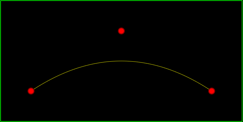
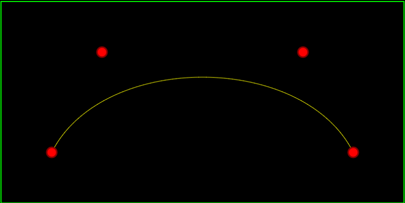
As you probably know, there is a tangent vector at every point on a curve (let’s ignore things like asymptotes for now), and the tangent vector basically points from one point on the curve to the next point on the curve. The tangent vector can also be seen as a slope of that point on the curve.

A gradient vector is another property of a point, but it is different than a tangent vector in a couple ways. First off, it is perpendicular to the tangent vector, so sticks out away from the curve, and could be seen as a normal vector. Secondly, every point in the graph has a gradient vector, even if that point isn’t part of the curve and is just floating by itself in empty space.

The interesting part here is that a gradient vector of a point not on the curve will actually lead you straight to the closest point on the curve to the point. This is because of a handy property where the line connecting a point to the closest point on the curve will be perpendicular to the curve (perpendicular to the tangent).

So, if we can calculate a gradient vector for a point, we have the vector that points towards the closest point on the curve. Technically it might be pointing away from the closest point on the curve, instead of towards it but that gets cleared up in the math.

Calculating Gradient Vector

The gradient vector is just a partial derivative for each of the variables of the equation. If you have no idea what I’m talking about, here are 2 options:

1) You can watch some videos and learn about it here: Khan Academy: Multivariable calculus
2) You can have wolfram alpha calculate it for you, by typing “gradient” before the function. Click this link to see what I mean: Wolfram Alpha: gradient x^2-y

Here are some example equations, along with their gradient vector, to make sure that you either understand what’s going on, or are properly entering your equations into wolfram alpha. Note that a gradient vector may not always be constant, in which case, it changes value for each point! If it is constant, it’s the same gradient vector across the entire graph space.

line:
f(x,y) = 2x – y
gradient(x,y) = (2, -1)

cubic function:
f(x,y) = x^3 – 10y
gradient(x,y) = (3x^2, -10)

sine:
f(x,y) = sin(x) – y
gradient(x,y) = (cos(x), -1)

circle:
f(x,y) = x^2 + y^2 – 5
gradient(x,y) = (2x, 2y)

Calculating Distance

Ok, so now that we have the value of our equation at some point (x,y) and we have the ability to find our gradient vector at that point, we have everything we need to calculate the distance from the point to the closest point on the curve.

All you need to do is divide the absolute value of the equation value at that point by the length of the gradient vector at that point.

Example 1 – Line

Let’s start with something super simple… y = x, aka x – y = 0 aka f(x,y) = x – y.

the gradient of that function is (1, -1) at every point on the graph. The magnitude of the gradient vector is the square root of 2.

What is the distance from the line to point P(2,0)?

Well.. the value of the equation at that point f(2,0) is 2, and the absolute value of that is still 2.

Next we divide that value by the magnitude of the gradient to get 2 / square root(2), which is just square root (2). So, the distance is square root of 2.

Since the value of the function at that point was positive before taking an absolute value, that means that the gradient points from the line to the point, so you can flip the gradient around to get (-1,1), and that is the direction that the closest point on the line is from the point P(2,0). If we travel square root of 2 units from P(2,0) down the vector (-1,1) we will get to the point (1,1) which is on the graph. That is the closest point on the graph to our point.

Note that it works out in this case, but usually the gradient vector won’t be the right magnitude since it’s not normalized. It happened that in this case it is, by dumb luck, but it usually isn’t.

Example 2 – Another Line

Let’s try a more complex line. y = 2x aka 2x – y = 0 aka f(x,y) = 2x – y.

the gradient of that function is (2, -1) with a magnitude of square root of 5 at all points on the graph.

What is the distance from that line to point P(1,5)?

Well, the value of the function at (1,5) is -3. When you take the absolute value of that, it becomes 3.

So, the distance is 3 / square root (5).

In this case, since the value of the function at the point was negative before we took the absolute value, it means that the gradient points from the point to the graph, so the line y=2x is 3/square root(5) units of length away from the point P(1,5) and the direction to travel from the point to get to the line is the same direction as the gradient vector at that point aka (2,1).

Example 3 – Quadratic Function

For the last example lets do y=x^2 aka x^2 – y = 0 aka f(x,y) = x^2 – y.

The gradient of that function is (2x,-1) and since it isn’t constant at all points, we can’t get the magnitude of the gradient yet.

What is the distance from that function to point P(2,0)?

Well, the value of f(2,0) is 4, which is still 4 if you take the absolute value.

The gradient at P(2,0) is (4,-1) with a magnitude of square root of 5.

So, the distance from point P(2,0) to the curve f(x,y) = x^2 – y is 4/square root(5) and to get from the point to the curve you should travel that distance down the same direction as the vector (4,-1).

Caveat

Ok ok… the other shoe dropping here is that this distance calculation is only a distance ESTIMATE, and not always the right answer.

This is because if the gradient is a constant or linear function, it will be correct, but higher order gradients don’t always follow straight lines from the point to the curve.

The good news though is that this estimation will be less than or equal to the actual distance. Maybe not as useful as a for sure distance calculation, but an upper bound estimate still has it’s uses (like in ray marching, or drawing vector graphics).

Basically, the straight line tells you the closest it could possibly be, but the actual gradient may take a longer, curving path, from the point to the curve.

More Info

Here’s the article that got me started down this path, trying to find the answer to this question, while trying to understand the main topic:
IQ: Distance Estimation

And here’s a link that really helped me understand what a gradient was, and what it was all about:
Vector Calculus: Understanding the Gradient

Khan academy videos about these topics:
Khan Academy: Multivariable calculus

Analytic Fog Density

AnalyticFog

There are a number of ways to implement the effect of fog with modern real time rendered graphics. This blog post will explain how to render fog that has varying density, based on a function of X,Y,Z location in space, like in the picture above.

Faked Fog

One way is to “fake it” and do something like set the color of a pixel on an object to be based on it’s height. For instance you might say that pixels with a y axis value above 15 are unfogged, pixels with y axis values between 15 and 10 progressively get more fogged as they get closer to 10, and pixels with y axis values less than 10 are completely fogged. That can make some fog that looks like this:

heightfog

A strange side effect of doing that though, is if you go down “into” the fog, and look out of the fog, things that should be fogged won’t. For instance, looking up at a mountain from inside the fog, the mountain won’t be fogged at all, even though it should be because you are inside of the fog.

A better way to do it, if you intend for the camera to be able to go into the fog, is to calculate a fogging amount for a pixel based on how far away it is from the view point, and how dense the fog is between the view point and the destination point.

If you are doing ray based rendering, like ray tracing or ray marching, you might find yourself trying to find how much fog is between points that don’t involve the view point – like if you are calculating the reflection portion of a ray. In this case, you are just finding out how much fog there is between the point where the reflection happened and the closest intersection. You can consider the point of reflection as the “view point” for the purpose of fogging.

Sometimes, the entire scene might not be in fog. In this case, you have to find where the fog begins and ends, instead of the total distance between the view point and the destination point.

In any case, the first thing you need to do when fogging is figure out the point where the fog begins, and the point where the fog ends. Then, you can figure out how much fog there is based on how the fog density works.

Constant Density Fog

GraphConstant

The simplest sort of fog is fog that has the same density all throughout it.

What you do in this case is just multiply the fog density by the distance spent in the fog to come up with a final fog value.

As an example, your fog density might be “0.04” and if you are fogging a pixel 10 units away, you multiply density by distance. FogAmount = 0.04 * 10.0 = 0.4.

Doing this, you know the pixel should be 40% fogged, so you interpolate the pixel’s color 40% towards the fog color. You should make sure to clamp the fog amount to be between 0 and 1 to avoid strange visual anomolies.

The image below shows a constant fog density of 0.04.

ConstantFog1

Here’s an image of the same constant density fog as viewed from inside the fog:

ConstantFog3

A problem with constant fog density though, is that if you view it from edge on, you’ll get a very noticeable hard edge where the fog begins, like you can see in the image below:

ConstantFog2

Linear Density Fog

GraphLinear

With linear fog density, the fog gets denser linearly, the farther you go into the fog.

With a fog plane, you can get the density of the fog for a specified point by doing a standard “distance from plane to point” calculation and multiplying that by how much the fog density grows per unit of distance. If your plane is defined by A*x+B*y+C*y+D = 0, and your point is defined as X,Y,Z, you just do a dot product between the plane and the point, giving the point a W component of one.

In other words…

FogDensity(Point, Plane) = (Plane.NormX * Point.X + Plane.NormY * Point.Y + Plane.NormZ * Point.Z + Plane.D * 1.0) * FogGrowthFactor

Here’s a picture of linear fog with a fog growth factor of 0.01:

LinearFog1

The same fog viewed from the inside:

LinearFog2

And lastly, the fog viewed edge on to show that the “hard line” problem of linear fog is gone (dramatic difference isn’t it?!):

LinearFog3

Analytic Fog Density – Integrals

GraphAnalytic

Taking a couple steps further, you might want to use equations to define fog density with some function FogDensity = f(x,y,z,).

How could you possibly figure out how much fog there is between two given points when the density between them varies based on some random function?

One way would be to take multiple samples along the line segment between the view point and the destination point, and either calculate the fog amount in each section, or maybe average the densities you calculate and multiply the result by the total distance. You might have to take a lot of samples to make this look correct, causing low frame rate, or accepting low visual quality as a compromise.

If you look at the graphs for the previous fog types, you might notice that we are trying to find the area under the graphs between points A and B. For constant density fog, the shape is a rectangle, so we just multiply width (time in fog) by height (the constant fog density) to get the fog amount. For linear density fog, the shape is a trapezoid, so we use the trapezoid area formula which is height (in this case, the distance in the fog) times the sum of the base lengths (the fog densities at points A and B) divided by 2.

How can we get the area under the graph between A and B for an arbitrary formula though? Well, a way exists luckily, using integrals (thanks to my buddy “Danny The Physicist” for educating me on the basics of integrals!).

There’s a way to transform a formula to get an “indefinite integral”, which itself is also a formula. I won’t go into the details of how to do that, but you can easily get the indefinite integral of a function by typing it into Wolfram Alpha.

Once you have the indefinite integral (let’s call it G(x)) of the fog density formula (let’s call it F(x)), if you calculate G(B) – G(A), that will give you the area under the graph in F(X) between A and B. Yes, seriously, that gives us the area under the graph between our points, thus giving us the amount of fog that exists between the two points for an arbitrary fog density function!

Note that when you plug a value into the indefinite integral and get a number out, that number is called the definite integral.

Analytic Fog Density – Implementation Details

Now that the theory is worked out let’s talk about implementation details.

First off, coming from an additive audio synthesis type of angle, I figured I might have some good luck adding together sine waves of various frequencies and amplitudes, so I started with this:

sin(x*F) * A

F is a frequency multiplier that controls how long the sine wave is. A is an amplitude multiplier that controls how dense the fog gets max.

Next, I knew that I needed a fog density function that never goes below zero, because that would mean if you looked through a patch of negative fog density, it would make the other fog you were looking through be less dense. That is just weird, and doesn’t exist in reality (but maybe there is some interesting visual effect hiding in there somewhere??), so the formula evolved to this, making sure the function never went below zero:

(1 + sin(x*F)) * A

Plugging that equation into wolfram alpha, it says the indefinite integral is:

(x – (cos(x*F)) / F) * A

You can check that out here:
Wolfram Alpha: (1 + sin(x*F)) * A.

It’s also kind of fun to ask google to graph these functions so you can see what they do to help understand how they work. Here are the graphs for A = 0.01 and F = 0.6:
Fog Density: graph (1 + sin(x*0.6)) * 0.01
Indefinite Integral: graph (x – (cos(x*0.6)) / 0.6) * 0.01

So, if you have point A and B where the fogging begins and ends, you might think you can do this to get the right answer:
FogAmount = G(B.x) – G(A.x)

Nope! There’s a catch. That would work if A and B had no difference on the y or z axis, but since they probably do, you need to jump through some hoops. In essence, you need to stretch your answer across the entire length of the line segment between A and B.

To do that, firstly you need to get that fog amount down to unit length. You do that by modifying the formula like so:
FogAmount = (G(B.x) – G(A.x)) / (B.x – A.x)

This also has a secondary benefit of making it so that your fog amount is always positive (so long as your fog density formula F(X) can’t ever go negative!), which saves an abs() call. Making it always positive ensures that this works when viewing fog both from the left and the right.

Now that we have the fog amount down to unit length, we need to scale it to be the length of the line segment, which makes the formula into this:
FogAmount = (G(B.x) – G(A.x)) * Length(B-A)/(B.x – A.x)

That formula will now give you the correct fog amount.

But, one axis of fog wasn’t enough to look very good, so I wanted to make sure and do one sine wave on each axis. I used 0.01 amplitude for each axis, but for the X axis i used a frequency of 0.6, for the Y axis i used a frequency of 1.2 and for the Z axis i used a frequency of 0.9.

Also, I wanted to give a little bit of baseline fog, so I added some constant density fog in as well, with a constant density of 0.1.

As a bonus, I also gave each axis a “movement factor” that made the sine waves move over time. X axis had a factor of 2.0, Y axis had a factor of 1.4 and Z axis had a factor of 2.2.

Putting all of this together, here is the final fog equation (GLSL pixel shader code) for finding the fog amount between any two points at a specific point in time:

//=======================================================================================
float DefiniteIntegral (in float x, in float amplitude, in float frequency, in float motionFactor)
{
	// Fog density on an axis:
	// (1 + sin(x*F)) * A
	//
	// indefinite integral:
	// (x - cos(F * x)/F) * A
	//
	// ... plus a constant (but when subtracting, the constant disappears)
	//
	x += iGlobalTime * motionFactor;
	return (x - cos(frequency * x)/ frequency) * amplitude;
}

//=======================================================================================
float AreaUnderCurveUnitLength (in float a, in float b, in float amplitude, in float frequency, in float motionFactor)
{
	// we calculate the definite integral at a and b and get the area under the curve
	// but we are only doing it on one axis, so the "width" of our area bounding shape is
	// not correct.  So, we divide it by the length from a to b so that the area is as
	// if the length is 1 (normalized... also this has the effect of making sure it's positive
	// so it works from left OR right viewing).  The caller can then multiply the shape
	// by the actual length of the ray in the fog to "stretch" it across the ray like it
	// really is.
	return (DefiniteIntegral(a, amplitude, frequency, motionFactor) - DefiniteIntegral(b, amplitude, frequency, motionFactor)) / (a - b);
}

//=======================================================================================
float FogAmount (in vec3 src, in vec3 dest)
{
	float len = length(dest - src);
	
	// calculate base fog amount (constant density over distance)	
	float amount = len * 0.1;
	
	// calculate definite integrals across axes to get moving fog adjustments
	float adjust = 0.0;
	adjust += AreaUnderCurveUnitLength(dest.x, src.x, 0.01, 0.6, 2.0);
	adjust += AreaUnderCurveUnitLength(dest.y, src.y, 0.01, 1.2, 1.4);
	adjust += AreaUnderCurveUnitLength(dest.z, src.z, 0.01, 0.9, 2.2);
	adjust *= len;
	
	// make sure and not go over 1 for fog amount!
	return min(amount+adjust, 1.0);
}

More Info

I ended up only using one sine wave per axis, but I think with more sine waves, or perhaps different functions entirely, you could get some more convincing looking fog.

At some point in the future, I’d like to play around with exponential fog density (instead of linear) where the exponential power is a parameter.

I also think that maybe squaring the sine waves could make them have sharper density changes perhaps…

One thing that bugs me in the above screenshots is the obvious “hard line” in both constant and linear fog where it seems fog crosses a threshold and gets a lot denser. I’m not really sure how to fix that yet. In traditional rasterized graphics you could put the fog amount on a curve, to give it a smoother transition, but in ray based rendering, that could make things a bit odd – like you could end up with an exponential curve butting up against the start of a different exponential curve (due to reflection or refraction or similar). The fog density would end up looking like log graph paper which would probably not look so great – although honestly I haven’t tried it to see yet!

If you have any questions, or feedback about improvements you know about or have discovered in any of the above, post a comment and let me know!

Here’s a good read on fog defined by a plane, that also gets into how to make branchless calculations for the fog amounts.
Unified Distance Formulas for Halfspace Fog

Interactive ShaderToy.com demo with GLSL pixel shader source code that you can also edit in real time with WebGL:
Fog

Feistel Networks – Do They Have to use XOR?

If you have no idea what a Feistel network is, but like cryptography and/or random number generation algorithms, read this link first:
Fast & Lightweight Random “Shuffle” Functionality – FIXED!

As a quick refresher, to encrypt data with a Feistel network, you break the plain text data into a left and a right side and do N rounds of this operation:

Left[i+1]  = Right[i];
Right[i+1] = Left[i] ^ RoundFunction(Right[i], key);

Where RoundFunction is ideally some chaotic function that returns some pseudo-random-esque number based on the inputs. For instance, RoundFunction could be MD5 so that it returned the MD5 hash of the data and the key, where the key could be considered the salt of the hash. The better the round function, the better your encryption algorithm will be.

To decrypt data with a Feistel network, you break the data into a left and right side and do the same number of rounds of this operation:

Right[i] = Left[i+1];
Left[i] = Right[i+1] ^ RoundFunction(Left[i+1], key);

Ok, onto the question….

Does it Have to use XOR?

Recently a friend of mine was using Feistel networks for something pretty amazing (so amazing, I can’t even talk about it), but in doing so, he asked me an interesting question. He asked “do you think this HAS to be XOR here, where we combine the round functions result back into the data?”. Well, it turns out, it doesn’t!

The operation has to be a reversible operation though, and you have to do the reverse operation when decrypting that you did while encrypting.

For instance, when encrypting you could add the round function result in, but then when decrypting, you would have to subtract the round function result out.

Or, you could do bitwise rotation left when encrypting, and right when decrypting perhaps.

Basically, anything that has a reverse operation can be used.

You have to be careful though because you might be lured into the trap of thinking that this includes something like multiplication and division.

If you multiply when you encrypt, you might get an integer overflow and lose data that can’t be corrected by doing a divide. For instance, if you multiply 255*2 in an unsigned 8 bit number you get 254 as a result. If you divide 254 by 2 to “undo” the multiplication, you get 127 which is obviously not 255, so we’ve lost some data. In an unsigned 8 bit number, ((255*2)/2) = 127.

If you go the other way and divide on encryption, and multiply on decryption, that doesn’t work either. For instance, when you divide 3 by 2, you get 1 with integer math, and when you multiply by 2, you get 2. So, with integers… ((3/2)*2) = 2.

Confusing note: you ARE able to do irreversible operations within the round function though. Feel free to do a divide or whatever you want in there. If that is difficult to understand how that could possibly work, you aren’t alone. Step through the code a bit by hand with a simple round function and a low number of rounds and you might be able to understand better how it does what it does.

I’m really not sure if anyone else out there does this variation on the traditional Feistel networks or not, but it is pretty interesting to combine the RoundFunction result back into the data with something other than XOR.

Source Code

Here’s some simple C++ code below to play with if you want to mess around with this stuff.

#include 
#include 
#include 

static const unsigned int c_numRounds = 4;

void PrimeRandomNumberPump ()
{
	// if you are curious about this, check out:
	// https://blog.demofox.org/2013/06/18/wtf-rand/
	srand((unsigned)time(NULL));
	for (unsigned int index = 0; index < 20; ++index)
		rand();
}

unsigned char RoundFunction (unsigned char value, unsigned char key)
{
	// Not a particularly effective round function, but the round function
	// isn't the point of this code.
	// If you want a better round function, try plugging in a hash function
	// or another chaotic function that has big changes in output for
	// small changes in input.  Also, you could change c_numRounds to a
	// higher number if you want better encryption.
	return value + key | (value * key) + 3;
}

void Encrypt (unsigned char &left, unsigned char &right, unsigned char key)
{
	for (unsigned int index = 0; index < c_numRounds; ++index)
	{
		// Feistel Network Encryption:
		//  Left[i+1]  = Right[i];
		//  Right[i+1] = Left[i] ^ RoundFunction(Right[i], key);

		// let's do addition to combine the value of the round function on 
		// encryption, instead of doing xor.  Xor is used in feistel networks
		// because xor is it's own inverse operation.
		unsigned char oldLeft = left;
		left = right;
		right = oldLeft + RoundFunction(right, key);
	}
}

void Decrypt (unsigned char &left, unsigned char &right, unsigned char key)
{
	for (unsigned int index = 0; index < c_numRounds; ++index)
	{
		// Feistel Network Decryption:
		//  Right[i] = Left[i+1];
		//  Left[i] = Right[i+1] ^ RoundFunction(Left[i+1], key);

		// let's do subtraction to combine the value of the round function on 
		// decryption, instead of doing xor.  Xor is used in feistel networks
		// because xor is it's own inverse operation.
		unsigned char oldRight = right;
		right = left;
		left = oldRight - RoundFunction(left, key);
	}
}

void DoTest (unsigned char plainText1, unsigned char plainText2, unsigned char key, int &tests, int &errors)
{
	// encrypt the plaintext
	unsigned char cipherText1 = plainText1;
	unsigned char cipherText2 = plainText2;
	Encrypt(cipherText1, cipherText2, key);

	// decrypt the cipher text
	unsigned char decryptedData1 = cipherText1;
	unsigned char decryptedData2 = cipherText2;
	Decrypt(decryptedData1, decryptedData2, key);

	// if the decrypted data doesn't match the plaintext data, count it as an error
	// and show the details
	tests++;
	if (decryptedData1 != plainText1 || decryptedData2 != plainText2)
	{
		errors++;
		printf("plaintext = 0x%02X%02Xrn", (unsigned int)plainText1, (unsigned int)plainText2);
		printf("ciphertext = 0x%02X%02Xrn", (unsigned int)cipherText1, (unsigned int)cipherText2);
		printf("decrypteddata = 0x%02X%02Xrnrn", (unsigned int)decryptedData1, (unsigned int)decryptedData2);
	}
}

void main (void)
{
	// generate a key
	PrimeRandomNumberPump();
	unsigned char key = (unsigned char)rand();

	// run tests with the key
	int errors = 0;
	int tests = 0;
	for (unsigned int y = 0; y < 256; ++y)
		for (unsigned int x = 0; x < 256; ++x)
			DoTest((unsigned char)y, (unsigned char)x, key, tests, errors);
		
	// display the test results
	printf("%i tests ran, %i errors encountered. key = 0x%02Xrn", tests, errors, key);
}

Bezier Curves Part 2 (and Bezier Surfaces)

This is a follow up post to Bezier Curves. My plan was to write a post about b-splines and nurbs next, but after looking into them deeper, I found out they aren’t going to work for my needs so I’m scratching that.

Here’s some basic info on b-splines and nurbs though before diving deeper into Bezier curves and surfaces.

B-Splines (Basis Splines)

Bezier curves are nice, but the more control points you add, the more complex the math gets because the degree of the curve function increases with each control point added. You can put multiple Bezier curves end to end to be able to have more intricate curves, but another option is to use B-Splines.

B-Splines are basically Bezier curves which let you specify more control points without raising the degree of the Bezier curve. They do this by having control points only affect part of the total curve.

This way, you could make a quadratic b-spline which had 10 control points. Only a few control points control any given point on the curve, so the curve stays quadratic (and so does the math), but you get a lot more control points. A “Knot Vector” is what controls which parts of the curve the control points control.

A Bezier curve is actually a special case of B-Spline where all control points affect the entire curve.

Nurbs (Non Uniform Rational B-Spline)

Sometimes when working with curves, you want some control points to be stronger that others. You can accomplish this in Bezier curves and B-splines by doubling up or trippling up control points in the same location to make that control point twice, or three times as strong respectively.

What if you want a control point to be 1.3 times stronger though? That gets a lot more complicated.

Nurbs solve that problem by letting you specify a weight per control point.

Just like Bezier curves are a special case of B-Splines, B-Splines are a special case of nurbs. A B-Spline could be thought of as nurbs that has the same weighting for all control points.

Back to Bezier!

My end goal is to find a curve / surface type that is flexible enough to be used to make a variety of shapes by artists, but is efficient at doing line segment tests against on the GPU. To this end, B-Splines and Nurbs add algorithmic and mathematical complexity over Bezier curves, and seem to be out of the running unless I can’t find anything more promising.

My best bet right now looks like a Bezier Triangle. Specifically, a quadratic Bezier triangle, where each side of the triangle is a quadratic Bezier curve that has 3 control points. When I get those details fully worked out, I’ll report back, but for now, here’s some interesting info I found about generalizing bezier curves both in order (linear, quadratic, cubic, quartic, etc) as well as in the number of dimensions (line, curve, triangle, tetrahedron, etc).

Bezier Generalized

I found the generalized equation on the wikipedia page for Bezier triangles and am super glad i found it, it is very cool!

I want to show you some specifics to explain the generalization by example.

Quadratic Curve:
(A * S + B * T) ^ 2

Expanding that gives you:
A^2 * S^2 + A * B * 2 * S * T + B^2 * T^2

In the above, S and T are Barycentric Coordinates in a 1 dimensional Simplex. Since we know that barycentric coordinates always add up to 1, we can replace S with (1-T) to get the below:

A^2 * (1-T)^2 + A * B * 2 * (1-T) * T + B^2 * T^2

Now, ignoring T and the constants, and only looking at A and B, we have 3 forms: A^2, AB and B^2. Those are our 3 control points! Let’s replace them with A,B and C to get the below:

A * (1-T)^2 + B * 2 * (1-T) * T + C * T ^2

And there we go, there’s the quadratic Bezier curve formula seen in the previous post.

Cubic Curve:
(A * S + B * T) ^ 3

To make a cubic curve, you just change the power from 2 to 3, that’s all! If you expand that equation, you get:
A^3*S^3+3*A^2*B*S^2*T+3*A*B^2*S*T^2+B^3*T^3

We can swap S with (1-T) to get:

A^3*(1-T)^3+3*A^2*B*(1-T)^2*T+3*A*B^2*(1-T)*T^2+B^3*T^3

Looking at A/B terms we see that there is more this time: A^3, A^2B, AB^2 and B^3. Those are our 4 control points that we can replace with A,B,C,D to get:
A*(1-T)^3+3*B*(1-T)^2*T+3*C*(1-T)*T^2+D*T^3

There is the cubic Bezier curve equation from the previous chapter.

Linear Curve:
(A * S + B * T) ^ 1

To expand that, we just throw away the exponent. After we replace S with (1-T) we get:
A * (1-T) + B * T

That is the formula for linear interpolation between 2 points – which you could think of as the 2 control points of the curve.

One more example before we can generalize.

Quadratic Bezier Triangle:
(A * S + B * T + C * U) ^ 2

If you expand that you get this:
A^2*S^2+2*A*B*S*T+2*A*C*S*U+B^2*T^2+2*B*C*T*U+C^2*U^2

Looking at combinations of A,B & C you have: A^2, AB, AC, B^2, BC, C^2. Once again, these are your control points, and their names tell you where they lie on the triangle. A Bezier triangle is a triangle where the 3 sides of the triangle are bezier curves. A quadratic bezier triangle has quadratic bezier curves for it’s edges which mean that each side has 3 control points. Those 3 control points are made up of the 3 corners of the triangle, and then 3 more control points, each one being between end points. A^2, B^2 and C^2 represent the 3 corners of the triangle. AB is the third control point for the bezier curve on the edge AB. BC and AC follow that pattern as well! Super easy to remember.

In a cubic Bezier triangle, you get a lot more control points, but a new class of control point too: ABC. This control point is in the middle of the triangle like the name would imply.

Anyways, in the expanded quadratic bezier triangle equation above, when you replace the control points with A,B,C for the triangle corner control points (the squares) and D,E,F for the inbetween control points, you get the bezier triangle equation below:

A*S^2+2*D*S*T+2*E*S*U+B*T^2+2*F*T*U+C*U^2

Note that we are dealing with a simplex in 3d now, so once again, instead of needing ALL Barycentric coordinates (S,T,U) we could pick one and replace it. For instance, we could replace U with (1-S-T) to have one less variable floating around.

All Done for Now

You can use this pattern to expand either in “surface dimension”, or in the dimension of adding more control points (and increasing the order of the equation). I love it because it’s super simple to remember that simple equation, and then just re-calculate the equation you need for whatever your specific usage case is.

If this stuff is confusing, check out the wiki page for Bezier Triangles, it has a great graphic that really shows you what I’m trying to explain:
Bezier Triangle

Next up I either want to make an HTML5 interactive app for messing around with Bezier triangles, or if I can figure out how to intersect a line segment with a quadratic Bezier triangle, i’ll probably just have some real cool looking screenshots to post along w/ the equation I ended up using (;

Special thanks to wolfram alpha for crunching some of these equations. Check it out, it’s really cool!
Wolfram Alpha – Cubic Bezier Curve Expansion

For more bezier fun check out my next Bezier post: One Dimensional Bezier Curves.

Implicit vs Parametric vs Explicit Surfaces

Implicit Surface

It’s always R = 0 where R is a function of one or more variables.

Like the unit circle equation:
x^2 + y^2 -1 = 0.

Parametric Surface

The components of the output are based on some parameter or parameters

Like the quadratic bezier curve (which A,B,C and CurvePoint are points in N dimensions):
CurvePoint = f(t) = A*(1-t)^2 + B*2t(1-t) + C*t^2

Or the unit circle:
x = cos(t)
y = sin(t)

Or surfaces like this:
SurfacePoint3D = f(u,v)

Explicit Surface

The more usual looking type functions where you have one variable on the left side (dependent variable), and another variable on the right side (independent variable).

Like lines:
y = mx + b

or height fields:
height = f(x,y)

More Info

Here’s a cool set of slides that explain this stuff in more detail (and beyond), and the pros and cons of using various forms.

Representing Smooth Surfaces

Bezier Surface Properties

Here’s a couple pretty cool properties of Bezier surfaces that I learned recently.

The first one is that if you consider a “convex hull” being made up of the control points (connect all the control points into a convex shape), the curve will lie entirely inside that shape. That means you can use the shape of the control points as a “quick test” for rendering or collision detection. Note though, you could also just make a sphere that enclosed all the control points and do a sphere test instead, if you would rather have a simpler/quicker test at the cost of some wasted space (more false positives).

The second interesting property is that you can do back face culling of a Bezier surface if all the control points face away from the camera. while it’s true this isn’t EXACTLY proper back face culling, the odds are good it’s good enough for your needs, especially given how quick a test it is.

The third interesting property is that if you want to transform a bezier surface with something like a translation, rotation, or scale, you can apply the transform to the control points, and the curve will be transformed by the same transformation.”A Bézier surface will transform in the same way as its control points under all linear transformations and translations.” (from Wikipedia: Bezier Surface)

… but unfortunately, as promising as these properties are, it still seems infeasible to render a decent number of bezier surfaces via real time raytracing (something i was planning on) and it seems to only get worse when moving to b-splines and nurbs surfaces, so it seems like this may not be the way to go. It’s still possible though that raymarching these surfaces could be doable, but I haven’t explored too much in that direction yet.

Bezier Curves

Bezier curves are pretty cool. They were invented in the 1950s by Pierre Bezier while he was working at the car company Renault. He created them as a succinct way of describing curves mathematically that could be shared easily with other people, or programmed into machines to make curves that matched the ones created by human designers.

I’m only going to go over bezier curves at the very high level, and give some links to html5 demos I’ve made to let you play around with them and understand how they work, so you too can implement them easily in your own software.

If you want more detailed information, I strongly recommend this book: Focus on Curves and Surfaces

Quadratic Bezier Curves

Quadratic bezier curves have 3 control points. The first control point is where the curve begins, the second control point is a true control point to influence the curve, and the third control point is where the curve ends. Click the image below to be taken to my quadratic bezier curve demo.


bezquad

A quadratic bezier curve has the following parameters:

  • t – the “time” parameter, this parameter goes from 0 to 1 to get the points of the curve.
  • A – the first control point, which is also where the curve begins.
  • B – the second control point.
  • C – the third control point, which is also where the curve ends.

To calculate a point on the curve given those parameters, you just sum up the result of these 3 functions:

  1. A * (1-t)^2
  2. B * 2t(1-t)
  3. C * t^2

In otherwords, the equation looks like this:

CurvePoint = A*(1-t)^2 + B*2t(1-t) + C*t^2

To make an entire curve, you would start with t=0 to get the starting point, t=1 to get the end point, and a bunch of values in between to get the points on the curve itself.

Cubic Bezier Curves

Cubic bezier curves have 4 control points. The first control point is where the curve begins, the second and third control points are true control point to influence the curve, and the fourth control point is where the curve ends. Click the image below to be taken to my cubic bezier curve demo.


bezcubic

A cubic bezier curve has the following parameters:

  • t – the “time” parameter, this parameter goes from 0 to 1 to get the points of the curve.
  • A – the first control point, which is also where the curve begins.
  • B – the second control point.
  • C – the second control point.
  • D – the fourth control point, which is also where the curve ends.

To calculate a point on the curve given those parameters, you just sum up the result of these 4 functions:

  1. A * (1-t)^3
  2. B * 3t(1-t)^2
  3. C * 3t^2(1-t)
  4. D * t^3

In otherwords, the equation looks like this:

CurvePoint = A*(1-t)^3 + B*3t(1-t)^2 + C*3t^2(1-t) + D*t^3

Math

You might think the math behind these curves has to be pretty complex and non intuitive but that is not the case at all – seriously! The curves are based entirely on linear interpolation.

Here are 2 ways you may have seen linear interpolation before.

  1. value = min + percent * (max – min)
  2. value = percent * max + (1 – percent) * min

We are going to use the 2nd form and replace “percent” with “t” but they have the same meaning.

Ok so considering quadratic bezier curves, we have 3 control points: A, B and C.

The formula for linearly interpolating between point A and B is this:
point = t * B + (1-t) * A

The formula for linearly interpolating between point B and C is this:
point = t * C + (1-t) * B

Now, here’s where the magic comes in. What’s the formula for interpolating between the AB formula and the BC formulas above? Well, let’s use the AB formula as min, and the BC formula as max. If you plug the formulas into the linear interpolation formula you get this:

point = t * (t * C + (1-t) * B) + (1-t) * (t * B + (1-t) * A)

if you expand that and simplify it you will end up with this equation:
point = A*(1-t)^2 + B*2t(1-t) + C*t^2

which as you may remember is the formula for a quadratic bezier curve. There you have it… a quadratic bezier curve is just a linear interpolation between 2 other linear interpolations.

Cubic bezier curves work in a similar way, there is just a 4th point to deal with.

Next Up

The demos above are in 2d, but you could easily move to 3d (or higher dimensions!) and use the same equations. Also, there are higher order bezier curves (more control points), but as you add control points, the computational complexity increases, so people usually stick to quadratic or cubic bezier curves, and just string them together. When you put curves end to end like that, they call it a spline.

Next up, be on the look out for posts and demos for b-splines and nurbs!

Soft Maximum vs Hard Maximum

The other day i stumbled on an interesting concept called a “Soft Maximum”.

If you think of the normal maximum, you might have something like this:

float maxValue = max(valueA, valueB);

if valueA and valueB come from functions, there’s usually going to be a sharp bend in the graph of the above where the maximum value changes from valueA to valueB or vice versa.

Sometimes, instead of a sharp bend, you would like a smooth transition between the two values – like when using this for graphics or advanced mathematics.

Here’s the formula for soft max:

double SoftMaximum(double x, double y)
{
	double maximum = max(x, y);
	double minimum = min(x, y);
	return maximum + log( 1.0 + exp(minimum - maximum) );
}

Here are 2 really interesting links on computing and using soft max:

Soft Maximum

How to Compute the Soft Maximum

Check out the images below for an example of when you might use this. This is from a shadertoy shader The Popular Shader. The first image is with using normal max, and the second image uses soft max.

softminOFF

softminON

Converting RGB to Grayscale

If you were converting an RGB pixel to grayscale, you might be like me and be tempted to just add the red, green and blue components together and divide by 3 to get the grayscale equivalent of the color.

That’s close, but not quite correct!

Red, green and blue are not equal brightness, so doing a straight average gives you biased results.

There’s a wikipedia page on this topic here, but the equation to use is below:
grayScale = red * 0.3f + green * 0.59f + blue * 0.11f;

Here are some sample images to show you the difference.

Color:
color

Average:
avg

Weighted Average Equation:
good

Why?

You might be wondering “why the heck would i want to convert RGB to grayscale?”

Well… if you render a scene once, convert it to grayscale and shove it into the red channel, then render the scene again slightly offset to the side, convert that to grayscale and shove it into the blue channel, you can get some neat images like the below. Red/Blue 3d glasses required, click the images to view the full size versions (;

Transformation Matrix Basics

Here are some interesting tidbits of info that I’ve found useful for being able to think about matrix math in a more intuitive way. We start off with 2d matrix math but extend it to 3d at the end.

Why Use A Matrix?

You might ask why you might go through all the trouble of using a matrix for doing transformations like translation, rotation, scaling and shearing / skewing.

Why not just manually modify the points, putting them through equations to get the results. Well, there are two main reasons.

The first one is for performance. The function for rotating a point in 2d looks like this:

x’ = x * cos(theta) – y * sin(theta)
y’ = x * sin(theta) + y * cos(theta)

If you have 1000 points, that means you are calculating sin twice and cos twice for each point which is 4000 trig operations. If you are smart (or your compiler is!), you’ll only do sin and cos once for each point, but that’s still 2000 trig operations.

If you are super duper smart (or your compiler is…), you’ll notice that theta is the same for all 1000 points, and perhaps you’ll calculate sin(theta) and cos(theta) once ahead of time and use those values for each point.

That last step is basically what matrix math does for you. A 2d rotation matrix looks like the below:

[ cos(theta), sin(theta) ]
[-sin(theta), cos(theta) ]

That means that once you have calculated your rotation matrix, you don’t need to keep performing trig operations. You have your values and can use them over and over very cheaply.

This especially saves processor time when you combine multiple transformations together. If you needed to perform an operation that did some crazy combination of 2000 rotations, 2000 translations and 2000 scale adjustments, instead of needing to do those 6000 operations on each point, you can just calculate the final matrix (by combining the matrix of each of those 6000 operations into one matrix) and then use that single matrix to your hearts content.

Another reason why you might want to use matrices instead of doing transforms by hand is that it’s a lot simpler writing code that does general transformations instead of deciding after the fact “hey i want to add scaling now and i need to touch all my transformation related code to implement it”.

Using a matrix, you don’t have to know or care what the transform is, it will just do it and you can move on with your life.

Matrix Vector Multiplication Is Just Dot Products!

As a quick refresher, in 2d, a dot product is just 2 multiplies and an add (A.X * B.X + A.Y * B.Y) and in 3d, a dot product is just 3 multiplies and 2 adds (A.X * B.X + A.Y * B.Y + A.Z * B.Z).

A lot of modern hardware (both CPU and GPU) has varying amounts of support built in for vector and matrix math to make it faster, but matrix vs vector multiplies are really not that bad to begin with. In 2d, a matrix * vector operation is just 2 dot products! In 3d, it’s 3 dot products. Look at the below to see what I mean:

[VX VY]
*
[AX AY]
[BX BY]
=
VX’ = AX * VX + BX * VY
VY’ = AY * VX + BY * VY

and in 3d:

[VX VY VZ]
*
[AX AY AZ]
[BX BY BZ]
[CX CY CZ]
=
VX’ = AX * VX + BX * VY + CX * VZ
VY’ = AY * VX + BY * VY + CY * VZ
VZ’ = AZ * VX + BZ * VY + CZ * VZ

You Can Make a Matrix From Basis Vectors

Let’s say that you are working in 2d and you want to rotate a point. Let’s say that for some reason you know what the rotated X and Y axis are supposed to be. You can actually create a rotation matrix from that knowledge alone without having to do any trig or geometry type math.

Like for instance, if you wanted an object’s x axis to point parallel to the vector of a moving object, and you knew the object’s normalized velocity vector (the direction it is moving, normalized to have a vector length of 1) was (0.34, 0.93).

That normalized velocity vector would be your X axis, and you could use the “faked 2d cross product” of flipping x and y and negating one to get a vector perpendicular to that X axis (aka your Y axis) . So…

X axis = ( 0.34, 0.93)
Y axis = (-0.93, 0.34)

(note, which one you negate on the Y axis matters only as much as you care which of the 2 directions you want the Y axis to point. Basically if you don’t care if it points up or down, it doesn’t matter which one you flip. If you do care, you need to pick the right one for the direction you want. This may not be the best way, but i do it by visual inspection, or by evaluating the math and seeing if it’s pointing in the way that i want or not. In other words… try it one way, and if it’s backwards, do it the other way.)

Now that we have an X and a Y axis, we just use the X axis as the first row, and the Y axis as the second row and get our rotation matrix:

[ 0.34, 0.93]
[-0.93, 0.34]

To see that it really works, try multiplying the vector (1,0) by that matrix to see if we get the right number out (it should be the same vector as the velocity of the object we are orienting to). We are basically verifying here that our X axis comes out to what it should.

[1 0]
*
[ 0.34, 0.93]
[-0.93, 0.34]
=
X’ = 0.34 * 1 – 0.93 * 0 = 0.34
Y’ = 0.93 * 1 + 0.34 * 0 = 0.93

now, let’s check our y axis

[0 1]
*
[ 0.34, 0.93]
[-0.93, 0.34]
=
X’ = 0.34 * 0 – 0.93 * 1 = -0.93
Y’ = 0.93 * 0 + 0.34 * 1 = 0.34

Note that when you put your X and Y axis basis vectors into the matrix, that they should be normalized, otherwise they will do strange things to your point – like introduce scaling and skewing.

You Can Get Basis Vectors From a Matrix

The process works backwards too which is really handy. If you have some matrix of unknown rotation, you can get the basis vectors out the same way you put them in.

You might have already seen this when looking at the matrix from the last example

[ 0.34, 0.93]
[-0.93, 0.34]

The first row (0.34, 0.93) is the X axis, and the second row (-0.93, 0.34) is the Y axis.

One caveat to be aware of though is that if you are working with a “matrix from the wild” where you don’t know if it’s a rotation matrix only, or if it might have some other transforms in it (scaling or skewing), the rows may not be normalized.

If you know for sure that it’s just a rotation matrix, you can take the basis vectors right out of the matrix. If you don’t know for sure, you need to normalize the basis vectors after you pull them out.

Why is this useful?

If in 3d, you had the matrix representing the camera transform, you could grab the 3rd row to get the forward vector. You could use this vector when launching a projectile from the player’s position so that it would go where they were aiming.

Again, in 3d if you had the camera matrix, you could grab the first row to get the “left vector” and you could add or subtract that from the player’s position to do strafing left and right.

No complex math required (:

2d Translation Matrix

To be able to have a matrix that can do translation, you need to go to a 3×3 matrix.

Below is what a translation matrix looks like. (TX,TY) is the translation.

[1 0 0]
[0 1 0]
[TX TY 1]

When you want to transform a 2d point by a 3×3 matrix like the above, you need to use a 1 for the Z component. Let’s see what happens when we transform a 2d point by this 3×3 translation matrix.

[X Y 1]
*
[1 0 0]
[0 1 0]
[TX TY 1]
=
X’ = X * 1 + Y * 0 + 1 * TX
Y’ = Y * 0 + Y * 1 + 1 * TY
Z’ = 1 * 0 + 1 * 0 + 1 * 1
=
X’ = X + TX
Y’ = Y * TY
Z’ = 1

If you want to transform a 2d VECTOR (something that represents a direction, not a location) by a 3×3 matrix, you need to use a zero in the Z component instead of a 1. You may have heard this before, but let’s see why:

[X Y 0]
*
[1 0 0]
[0 1 0]
[TX TY 1]
=
X’ = X * 1 + Y * 0 + 0 * TX
Y’ = Y * 0 + Y * 1 + 0 * TY
Z’ = 1 * 0 + 1 * 0 + 0 * 1
=
X’ = X
Y’ = Y
Z’ = 0

As you can see, the vector was not affected by the translation of the matrix. If the 3×3 matrix had scaling and rotation in it as well as the translation, the vector WOULD be affected by those things as it should be. The translation is the only thing that doesn’t apply when you use a Z value of zero.

Note that if you want to get the 2d basis vectors from a 3×3 matrix, you just ignore the 3rd row and the 3rd column and do the same thing you would do with a 2×2 matrix. Again, making sure to normalize the basis vectors when it’s appropriate.

Combining Matrices

To combine transforms together (whether 2×2 or 3×3 matrices) you just multiply them together.

The order of matrix multiplication matters though. A * B is not the same as B * A.

To make things confusing, OpenGL and DirectX use different representations of matrices (one is “column major” the other is “row major”) which means that the matrices in each API are transposes of the other.

To make things even more confusing, if AT and BT are the transpose of A and B, then A * B = BT * BA. This means that premultiplication and postmultiplication (aka is A on the left or the right in A * B) swap meanings when going from one API to the other.

I’m not sure who is to blame for that one, but here’s an interesting link on the subject: http://steve.hollasch.net/cgindex/math/matrix/column-vec.html

Note that row vs column major matrices also change which direction the basis vectors are stored in… so instead of X axis being the 3 top numbers, it would be the 3 left numbers! It should be easy enough to tell which is which by inspection, but keep it in mind!

Anyways, I’ll continue to use the conventions set in this article above in the vector / matrix multiplication.

If you multiply a translation matrix by a rotation matrix, you’ll get a matrix that rotates a point, and then translates it.

[1 0 3]
[0 1 5]
[0 0 1]
*
[ 0.34 0.93 0]
[-0.93 0.34 0]
[ 0 0 1]
=
[ 0.34 0.93 3]
[-0.93 0.34 5]
[ 0 0 1]

If, however, you multiply a rotation matrix by a translation matrix, you’ll get a matrix that translates a point, then rotates it. Going that direction, the translated point is rotated.

[ 0.34 0.93 0]
[-0.93 0.34 0]
[ 0 0 1]
*
[1 0 3]
[0 1 5]
[0 0 1]
=
[ 0.34 0.93 5]
[-0.93 0.34 1.4]
[ 0 0 1 ]

Which way you multiply entirely depends on what it is you are trying to achieve. And, well… it also depends on whether you are dealing with row major or column major matrices!

Multiplying a 3×3 matrix by another 3×3 matrix is the same as doing nine 3d dot products.

Inverting Matrices

Taking the transpose of a matrix doesn’t have any intuitive geometrical (or other) meaning that I’m aware of. I’ve looked on the net and all I could find was some “simple” explanations involving general relativity. Awesome right? LOL.

On the other hand, inverse matrices have a very intuitive and very useful meaning. Inverse matrices do the reverse of whatever the matrix does.

That means if you have a matrix that translates by (7,5) and then rotates by (45, 30) degrees, the inverse matrix will rotate by (-45, -30) degrees and then translate by (-7,-5).

This is super useful sometimes (:

Inverting a 2×2 matrix is actually really easy. I could explain it but you really ought to check out this page to see how. I recommend doing the exercises at the bottom to make sure you firmly understand how to do it!

http://www.mathsisfun.com/algebra/matrix-inverse.html

Inverting a 3×3 matrix is fairly easy too, but kind of tedious. Here’s a page that explains how:
http://www.wikihow.com/Inverse-a-3X3-Matrix

After you are done with that, here are some problems to run through to make sure you really do understand it:
https://www.khanacademy.org/math/algebra/algebra-matrices/inverting_matrices/e/matrix_inverse_3x3

Not all matrices are invertible. If you read the links and walk through the exercises, you’ll see why. Basically, an uninvertable matrix will cause a divide by zero in the inversion process. I believe this comes up when you have a matrix with parallel basis vectors, or if you have a zero scaling matrix (a multiply by zero can’t be reversed!) but i could be mistaken or not have the full picture there. If I’ve mis-spoken, post a comment!

Extending to 3d

Extending the above to 3d matrices is pretty simple and there aren’t really many suprises.

One difference is that in the above where we use a 2×2 matrix in 2d, we would use a 3×3 matrix in 3d because of the extra Z coordinate.

If you want to do translation in 3d, you have to use a 4v4 matrix instead of a 3×3 (just like in 2d how you had to move from a 2×2 to a 3v3, in 3d you have to move from a 3×3 to a 4×4). A 3d translation matrix looks like this:

[1 0 0 0]
[0 1 0 0]
[0 0 1 0]
[TX TY TZ 1]

Inverting a 4×4 matrix is pretty tedious, but follows the same patterns as inverting a 3×3 and a 2×2.

You can find info on a 3d rotation matrix here, if you don’t want to build it up with basis vectors: http://en.wikipedia.org/wiki/Rotation_matrix#In_three_dimensions

In our example above where we had the X axis and used a “fake 2d cross product” to get the perpendicular vector, when you move into 3d you’ll probably want to use the cross product to get perpendicular vectors.

Like for instance if you know 2 of the basis vectors, you can use cross product of those 2 to get the third.

Z = X x Y

If, however, you only have one basic vector (say “Z” because maybe you have a “camera direction”), you can use cross product to get 2 other vectors so long as you can make certain assumptions about the orientations involved. Like for instance, you might do this:

Fwd = normalize(Camera.Forward)
Left = normalize(Fwd x (0, 1, 0))
Up = normalize(Fwd x Left)

rotation matrix =
[Left.X Left.Y Left.Z]
[Up.X Up.Y Up.Z]
[Fwd.X Fwd.Y Fwd.Z]

The above only works if the camera can never look straight up, and it also assumes that your camera doesn’t have any roll – but it is a useful technique if those assumptions are ok.

That’s about it! I hope you found at least some of this information useful (:

if I missed anything you think belongs here, post a comment and share with the rest of us!

Converting To and From Polar / Spherical Coordinates Made Easy

As a game developer there is just too much darn stuff to learn. You could spend your entire life learning things and never know it all.

It’s a blessing in that you are seldom bored, but also sometimes a curse in that there almost always is a better way to do something, and that you would know about it if you had spent your time learning X instead of Y 😛

I find that you sort of have to triage what you learn and what you choose to keep fresh in your mind, which can be a challenge sometimes. If you can find the commonalities between things that can help some – like understanding how encryption, hashing, pseudo random number generators and chaos theory all overlap – or how skeletal animation blending and audio synthesis are both trying to be continuous waves above all else. Also, if you put in the time investment to learn something to where it becomes intuitive, that frees up neurons to make room for other stuff. But, of course, we have a finite amount of time, so can’t always spend the time needed to get to that level on every single topic.

How about you… do you have to do a juggling act like this to keep sharp and stay effective as a game (or non-game) programmer? I’d be interested to hear how others deal with this sort of thing with such a large knowledge space that we work in.

In any case, I usually work with spherical or polar coordinates only on rare occasions, so whenever i do, the process usually is to google the equations, drop them in, and move on with my life. I was recently implementing an orbit camera for a raytracer on shadertoy.com (Raytraced Refraction) and when my copy/pasting wasn’t working, I was forced to take a deeper look at why it wasn’t working. Amazingly, this time around, it finally clicked and is now an intuitive thing so I figured I’d share the explanation that makes most sense to me in case it helps anyone else.

Converting Polar Coordinates to Cartesian (2D)

Polar coordinates have two components – a distance and an angle – and represent a point in 2d space.

The distance is called the radial coordinate, or the radius and the angle is called the angular coordinate or polar angle.

Just like you probably expect, the angle defines what direction the point is in, and the radius defines how far away it is. Super simple. Below is a picture of a polar coordinate point at (3, 45) where 3 is the distance and 45 is the angle.

polar1

So how do we convert that to rectangular coordinates? well, first thing to do is to convert the angle to rectangular coordinates on a unit circle to get a direction vector. Then, you multiply that direction vector by the radius to get the final coordinate.

To convert the angle to a point on a unit circle and get the direction vector it’s super simple…

X = cos(angle)
Y = sin(angle)

For every point on the unit circle, it’s X coordinate is the cosine of the angle, and it’s Y coordinate is the sine of the angle.

Looking at the diagram below, see if you can figure out why arccosine only returns an angle between 0 and 180, and why arcsine only returns an angle between -90 and 90 (hint, what if i asked you to tell me what angle gives 0.7 in the x component). Also see if you can understand why sin(x)^2 + cos(x)^2 = 1 (hint: distance formula).

polcorunitcircle

Ok so now that we can get our direction vector, we just need to multiply it by the radius. So… to convert from polar to rectangular (cartesian) coordinates, you do this:

X = cos(angle) * radius
Y = sin(angle) * radius

Converting Cartesian to Polar Coordinates (2D)

So how do we convert from rectangular coordinates to polar?

Well, since we have the X and the Y coordinates, and we know that tangent(angle) = Y / X, we can use arctangent to get our angle. Unfortunately atan has a similar problem to asin and acos in that it doesn’t know which quadrant you are talking about. For instance, look at the diagram above again and tell me “which angle gives me a value of 1 when i divide the Y component by the X component?”. The answer is 45 degrees and 225 degrees both. This is because with a positive value of 1, we don’t know if X and Y were both negative, or if they were both positive. Similarly, if i asked which angle gave an answer of -1, we wouldn’t know if it was the X or Y that was negative.

Instead of using atan, we want to use atan2, which takes 2 parameters – Y and X – so that it can figure out the correct angle for you.

Next is the easy part of finding the radius. treating your point as a vector (or continuing to treat it like a vector if it IS a vector), the radius is just the magnitude of the vector (or distance from the origin if you want to think of it in “point” terms instead of vectors).

So, converting rectangular to polar coordinates is done like this:

radius = sqrt(X * X + Y * Y)
angle = atan2(Y, X)

Converting Spherical Coordinates to Cartesian (3D)

Spherical coordinates have the same components as polar coordinates, but then an added component: an angle which determines pitch / vertical rotation (think: looking up and looking down, instead of the polar angle which is in charge of looking left and right).

In math, they usually call the radius rho, the polar angle theta, and the azimuth angle phi, so a formal polar coordinate looks like this:

(rho, theta, phi)

For our examples let’s assume that X and Y make up the horizontal plane and that Z is the vertical (3d) axis.

If you are scared to make the jump from 2D polar coordinates to 3D spherical coordinates don’t be! The way to deal with these guys is to break the 3d problem into two 2d problems, using the exact same stuff as described above.

So, the first thing we want to do is completely ignore this new 3rd component phi and think back to our 2d case. We are also going to ignore the radius for now.

XTheta = cos(theta)
YTheta = sin(theta)

This is our direction vector on the horizontal plane (same as the 2d case, not accounting for radius yet).

Next we want to pretend like we are looking at our 3d world from the side and use our phi angle to convert from polar to rectangular coordinates:

XPhi = cos(phi)
YPhi = sin(phi)

One way to think of what this other angle phi means, is that it is controlling where in the unit sphere the theta circle sits. As the theta circle gets higher or lower on the sphere, it shrinks or grows. It’s only at zero angle that it has a radius of 1.0. So, calculating these values, YPhi represents how high on the sphere the theta circle should sit, and XPhi is how large the circle should be.

So, to combine the X,Y theta values and the X,Y Phi values, we use YPhi as the vertical component, and XPhi as a radius for the theta circle, which we can do like this:

X = XTheta * XPhi
Y = YTheta * XPhi
Z = YPhi

The above equation will give us a point on a unit sphere, so from here, we need to multiply in the radius and our equation becomes:

X = XTheta * XPhi * radius
Y = YTheta * XPhi * radius
Z = YPhi * radius

If we put sin and cos back in, instead of xtheta (etc), the equation becomes that familiar, and previously complex equation:

X = cos(theta) * cos(phi) * radius
Y = sin(theta) * cos(phi) * radius
Z = sin(phi) * radius

Hopefully the equation makes more sense now, and hopefully you can look at that and intuitively understand why those values are what they are.

Converting Cartesian to Spherical Coordinates (3D)

To convert from spherical coordinates to rectangular, the first thing to do is to get the radius, which is done in the exact same way as in 2d. We just take the magnitude of the vector (aka the distance of the point from the origion) and we are done.

To get theta and phi, we do the same thing of separating this 3d problem into two 2d problems.

In fact, to get theta, we do the exact same thing as we do for polar coordinates! We use atan2(Y,X) to get our angle… THAT’S ALL!

So, we have this so far:

radius = sqrt(X * X + Y * Y + Z * Z)
theta = atan2(Y, X)

How do we figure out phi? Well, if you said that we should do atan2(Z,Y) or atan2(Z,X) you were pretty close but it’s actually arccos(Z / radius).

The reason for this is because neither X, nor Y is the “X” component of the “phi 2d polar coordinate”. you’d have to take the length of the (X,Y) vector and use that if you wanted to use atan2 to calculate phi. Instead of calculating that vector length, we can instead use a value we already have. cosine is Y / hypotenuse length, and hypotenuse length is the radius (length of our vector), so we might as well use that radius we already have to be able to use arccos.

The final equations for converting rectangular to spherical are:

radius = sqrt(X * X + Y * Y + Z * Z)
theta = atan2(Y, X)
phi = acos(Z / radius)

More info / alternate forms available on wikipedia here:
From Cartesian to Spherical Coordinates
Spherical Coordinate System