While it’s true that the GPU texture sampler can evaluate digital logic circuits, it turns out there’s a much better and simpler way to evaluate logic with textures. That better and simpler way isn’t even that useful unfortunately!

This post will show the path I took from the initially intriguing possibilities to the more mundane final answer. You may be able to see mistakes in my reasoning along the way, or be able to get to the punch line sooner (:

This was meant to be an extension to a paper I wrote talking about how you can evaluate Bezier curves by storing only the control points in a texture and then sampling along the texture diagonal:
GPU Texture Sampler Bezier Curve Evaluation

The ideas from this post started with a tweet from @marcosalvi:

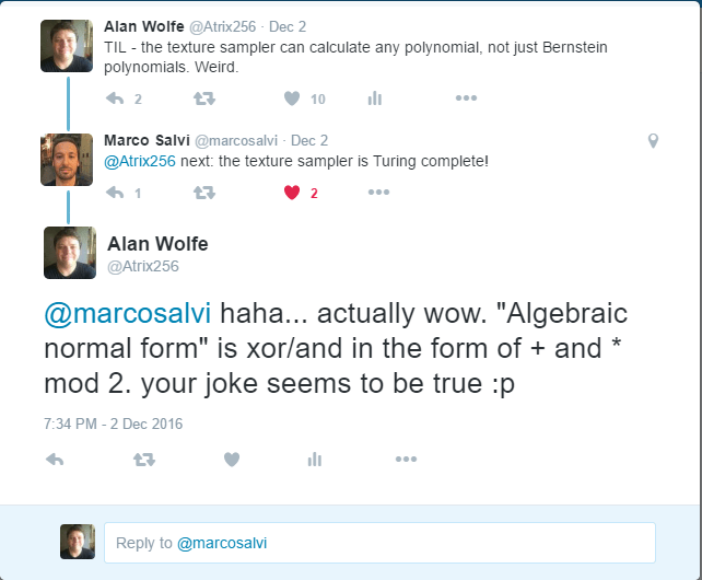
Because the last post showed how to evaluate arbitrary polynomials using the texture sampler, and digital circuits can be described as as polynomials in Algebraic Normal Form (ANF), that means we can use the texture sampler to evaluate digital logic circuits. Let’s check it out!

First up, we need to be able to convert logic into ANF. Oddly enough, I already have a post about how to do that, with working C++ source code, so go check it out: Turning a Truth Table Into A digital Circuit (ANF).

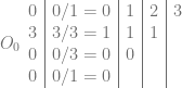
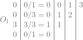
As an example, let’s work with a circuit that takes 3 input bits, and adds them together to make a 2 bit result. We’ll need one ANF expression per output bit. will be the 1’s place output bit (least significant bit), and will be the 2’s place output bit (most significant bit). Our 3 input bits will be u,v,w.

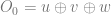
If we want to use our polynomial evaluation technique, we need equations that are univariate (one variable) instead of multivariate (multiple variables). We can try just using a single variable x in place of u,v and w. Remember that in ANF, you work with polynomials mod 2 (aka ), and that XOR () is addition while AND is multiplication. This gives the formulas below:

The next thing we need to use the technique is to know the Bezier control points that make a Bezier curve that is equivalent to this polynomial. Since we have 3 input variables into our digital circuit, if they were all 3 multiplied together (ANDed together), we would have a cubic equation, so we need to convert those polynomials to cubic Bernstein basis polynomials. We can use the technique from the last post to get the control points of that equivalent curve.

Now that we have our control points, we can set up our textures to evaluate our two cubic Bezier curves (one for , one for ). We’ll need to use 3d textures and we’ll need to set up the control points like the below, so that when we sample along the diagonal of the texture we get the points on our curves.

The picture below shows where each control point goes, to set up a cubic Bezier texture. The blue dot is the origin (0,0,0) and the red dot is the extreme value of the cube (1,1,1). The grey line represents the diagonal that we sample along.

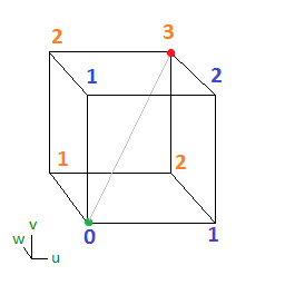
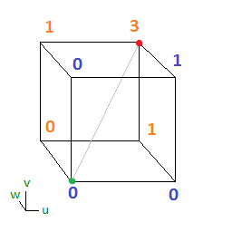
Coincidentally, our control points for the curve are actually 0,1,2,3 so that cube above is what our 3d texture needs to look like for the curve.

Below is what the curve’s 3d texture looks like. Note that in reality, we could store these both in a single 3d texture, just use say the red color channel for and the green color channel for .

Now that we have our textures set up let’s try it out. Let’s make a table where we have our three input bits, and we use those as texture coordinates in our 3d textures (the texture cubes above) to see what values we get. (Quick note – things are slightly simplified here vs reality. The pixel’s actual value is at a half pixel offset from the texture coordinates, so we’d be sampling between (0.5,0.5,0.5) and (1.5,1.5,1.5) instead of from (0,0,0) to (1,1,1), but we can ignore that detail for now to make this stuff clearer.)

Now, let’s modulus the result by 2 since ANF expects to work mod 2 ( to be more precise), and put the decimal value of the result next to it.

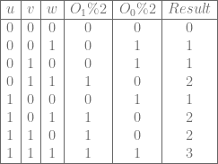
It worked! The result value is the count of the input bits set to 1.

Unfortunately we have a problem. When we converted the multivariate equation into a univariate equation, we just replaced u,v,w with x. This is only valid if the function is symmetric – if u,v,w can be interchanged with each other and not affect the result of the function. This bit adding digital circuit we made happened to have that property, but most digital circuits do not have that property – most of the time, not all input bits are treated equal. If we made a circuit that added two 2-bit numbers and have a 3-bit result for instance, the high bits of the input numbers have a very different meaning than the low bits and this technique falls apart. (Quick note – we are actually doing the reverse of the polynomial blossoming thing i mentioned in the last post. Blossoming is the act of taking a univariate function and breaking it into a multivariate function that is linear in each variable. The term is called symmetric multiaffine equation if you want to find out more about that.)

This turns out not to be a deal breaker though because it turns out we didn’t have to do a lot of the work that we did to get these volume textures. It turns out we don’t need to calculate the Bezier curve control points, and we don’t even need to make an ANF expression of the digital circuit we want to evaluate.

Let’s recap what we are trying to do. We have 3 input values which are either 0 or 1, we have a 3d texture which is 2x2x2, and we are ultimately using those 3 input values as texture coordinates (u,v,w) to do a lookup into a texture to get a single bit value out.

Here’s a big aha moment. We are just making a binary 3d lookup table, so can take our truth table of whatever it is we are trying to do, and then directly make the final 3d textures described above.

Not only does it work for the example we gave, with a lot less effort and math, it also works for the broken case I mentioned of the function not being symmetric, and not all input bits being equal.

Something else to note is that because we are only sampling at 0 or 1, we don’t need linear texture interpolation at all and can use nearest neighbor (point) sampling on our textures for increased performance. Also because the texture data is just a binary 0 or 1, we could use 1 bit textures.

The second aha moment comes up when you realize that all we are doing is taking some number of binary input bits, using those as texture coordinates, and then looking up a value in a texture.

You can actually use a 1D texture for this!

You take your input bits and form an integer, then look up the value at that pixel location. You build your texture lookup table using this same mapping.

So… it turns out this technique led to a dead end. It was just extra complexity to do nothing special.

Before it all fell apart, I was also thinking this might be a good avenue for doing homomorphic encryption on the GPU, but I don’t believe this aids that at all. (Super Simple Symmetric Leveled Homomorphic Encryption Implementation)

But Wait – Analog Valued Logic?

One thought I had while all this was unraveling was that maybe this was still useful, because if you put an analog value in (not a 0 or 1, but say 0.3), that maybe this could be used as a sort of “Fuzzy Logic” type logic evaluation.

Unfortunately, it looks like that doesn’t work either!

You can see how it breaks down and some more info here:
Computer Science Stack Exchange: Using analog values with Algebraic Normal Form?

Oh Well

Sometimes when exploring new frontiers (even if they are just new to us) we hit dead ends, our ideas fail etc. It happens. It’s part of the learning process, and also is useful sometimes to know what doesn’t work and why, instead of just always knowing what DOES work.

Anyways… posts on using the texture sampler for calculating points on data surfaces and data volumes are coming next (:

To give a brief taste of how that is going to play out:

• Doing a single texture read of a 3d RGBA texture can give you a triquadratic interpolated value.
• Alternately, doing a single texture read of a 3d RGBA texture can give you a bicubic interpolated value.

Thanks for reading!