
Prefix sums and summed area tables let you sum up regions of arrays or grids in constant time.
If that sounds like it might not have many uses, that is another way of saying that it does discrete integration in constant time, and can also be made to do some kinds of convolution.
These things come up quite a bit in game development and graphics so is pretty interesting for things like depth of field, glossy reflections, and maybe image based lighting. Check the links at the end of the post to see these things in action in some pretty interesting ways.
We’ll start with one dimension.
One Dimension – Prefix Sums
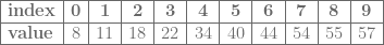
Say that you have 10 numbers:

To sum up numbers in a given range you have to manually add up the numbers in that range.
Summing the numbers at index 2 through 5 inclusively takes 3 adds and gives you the answer 29. (index 2 + index 3 + index 4 + index 5)
Summing the numbers at index 0 through index 9 inclusively (the whole table) takes 9 adds to get the answer 57.
Interestingly there is a way to preprocess this data such that summing any range takes only a single subtraction. The technique is called a prefix sum table and you make the table by having the number at each index be the sum from index 0 to that index inclusively.
Here is the prefix sum table for the numbers above:
Now, to find the sum of range a to b inclusively, you start with the value at index b, and subtract the value at index (a-1).
So, to sum the numbers at index 2 through 5 like we did before, we’d start with the value at index 5 which is 40, and we subtract the value at index (2-1) aka index 1, which is 11. That gives us a result of 29 like our manual summing did before.
To sum the numbers at index 0 through index 9, we’d start with the value at index 9, which is 57, and subtract the value at index -1. Since we don’t have anything before index 0, the sum for anything before index 0 is 0. That makes our result be 57-0 or 57, which we calculated before.
Let’s move on to 2D!
Two Dimensions – Making a Summed Area Table
In two dimensions, the same technique is called a summed area table, and things get only a little more complicated.
You start with a 2d grid of values like this:
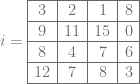
Then you make a grid of the same size, where the value at a location is the sum of all the values in the rectangle going from (0,0) to (x,y) inclusive. Assuming that (0,0) is in the top left, that would give us this summed area table:
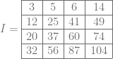
You can literally sum up all the values for each index to make the table if you want to, but you can also use this formula which lets you iteratively create the table by starting at (0,0) and expand outwards from there. As before, when reading out of bounds values, just use zero.

Two Dimensions – Using a Summed Area Table
So we know that 


With some cleverness we can calculate the sum inside this exact region.
First we get the value at point D, which gives us the sum of this rectangle:

Next, we subtract the value at point B, which gives us the sum of this rectangle:

The next step is to subtract the value at point C. The red area is a problem though as it has been subtracted out twice.

This is a problem that’s easily solved by adding the value at point A in, to give us our final result:

So, to summarize, using a summed area table to get the sum of all values in the rectangle defined by the points A,B,C,D is done by reading the values at points A,B,C,D and calculating: A+D-B-C
Storage Costs
When you want to store numbers added together, you are going to need storage larger than what you are storing the numbers in.
For instance, if you have the table below using 3 bits per value:

Turning that into a summed area table, you are going to hit overflow problems:

For summing up N items, you need 

On twitter, Sam Littlewood (https://twitter.com/samlittlewood) shared some interesting info with me:
Using the previously shown 2×2 table of 3bit 7’s as an example, what this means is that if you are only ever going to want to ask about 1×1 ranges (which is pointless to use summed area tables for, but makes a nice simple example), you don’t need 2 extra bits, and in fact don’t need any extra bits in this case since a 1×1 range is just 1 sample, and 
Looking back at the summed area table that had roll over problems:
Let’s ask about the range (1,1) to (1,1). So we start with the value at index (1,1) which is 4. Next we add in the value at index (0,0) which is 7 and get 11. Keeping that in 3 bits (eg mod 8), that gives us a value of 3. Next we subtract the value at index (0,1) aka 6, which keeping it in 3 bits gives us 5. Subtracting index (1,0) from that (6 again) and keeping it in 3 bits gives us 7.
So, the sum of the numbers from (1,1) to (1,1) – aka the VALUE in the original table at (1,1) – is 7. Since we made the table, we know this is correct.
It works interestingly!
If we did a 2×2 lookup instead, it would fall apart. we’d need those 2 extra bits since we’d be summing 4 samples, and 
So, just to re-iterate… summed area tables do need increased storage per data item to store the sums. However, while most descriptions base that increased storage on the size of the image being made into a summed area table, it is actually based on the largest range you want to sum from that table, which may be smaller than the total size.
I have an idea I’d like to try (next blog post?) where instead of storing the sum of the rectangle at each position, you store the sum divided by the area. In other words, you store the average value for the rectangle.
Calculating the sum for a specific rectangle then becomes getting the 4 values, multiplying by their area, and then doing the usual math.
Apparently this is similar to an idea of using floating point numbers in SAT, which also sounds interesting! Thread from Bart Wronski (https://twitter.com/BartWronsk):
While my idea is similar to using floating point, a handful of people (especially Tom Forsyth! https://twitter.com/tom_forsyth) have made sure I know that using floating point with large textures (~screen sized and above) is not a good idea.
Tom says:
“The entries in the bottom-right of the table start having very similar magnitudes, so the difference between them is very noisy. This is super obvious with float16s where you only have 10 bits of precision, which is less than most current screen widths.”
Other Stuff
Bilinear Interpolation
If you are wondering whether you should use bilinear interpolation when using this technique (sample between pixels) or not, the answer is that you should. Bilinear interpolation is compatible with this technique and gives you the correct values for sub pixel sample points.
Higher Dimensions
This technique extends to 3 dimensions and beyond. The table still contains the sum of the numbers for the (hyper)rectangle from the origin to that specific index. The way you calculate the sum of a specific range is different in each dimension, but it’s similar, and you should be able to figure it out using the logic described in the 2d case!
Integrating / Summing Over Other Shapes
I had a thought on this that might not be so bad.
My thought was that if you had some shape you wanted to sum values over (aka integrate values over), that you could sum over the bounding box of the shape, divide by the area of the bounding box to get an average sum per unit for that area, and then multiply by the area of the shape you want to sum over.
This makes the assumption that the bounding box is representative of the data inside of the shape, so that makes this an approximation, but it might be good enough depending on your needs.
You might even try having a couple different summed area tables made from rotated versions of the image. That would allow you to get a tighter fitting bounding box in some situations.
I’m definitely not the first to think about how to do this though, and this is not the only way to do it. There is a link in the next section that talks about a different way to do it “Fast and Exact Convolution With Polygonal Filters” that also references a few other ways to do it.
Uses in Graphics / Other Links
Here is the paper from Franklin Crow in 1984 that introduces summed area tables as a way to get box filtered mipmapping on the fly without having to generate mipmaps in advance:
Here is a neat paper that talks about how to generate summed area tables efficiently on the GPU, and some interesting ways to use them for things like depth of field, glossy reflections, and refraction through frosted glass:
http://citeseerx.ist.psu.edu/viewdoc/download?doi=10.1.1.90.8836&rep=rep1&type=pdf
Here are some great reads from Fabien Giesen (https://twitter.com/rygorous) on doing fast blurs when the radius is very large. The second post also shows you how to do repeated box blurs to get tent filters, quadratic filters, cubic, etc and how they tend towards Gaussian. I’m sure there is some way to mix this concept with summed area tables to get higher order filters, but I haven’t found or worked out the details yet.
https://fgiesen.wordpress.com/2012/07/30/fast-blurs-1/
https://fgiesen.wordpress.com/2012/08/01/fast-blurs-2/
Here are some blog posts I made up explaining and demonstrating box blurs and Gaussian blurs:
https://blog.demofox.org/2015/08/18/box-blur/
https://blog.demofox.org/2015/08/19/gaussian-blur/
Bart also shared these really interesting links
“Fast and Exact Convolution With Polygonal Filters”
https://www.researchgate.net/publication/269699690_Fast_and_Exact_Convolution_with_Polygonal_Filters
“Fast Filter Spreading and its Applications”
Click to access EECS-2009-54.pdf
“Filtering by repeated integration”
https://www.researchgate.net/publication/220721661_Filtering_by_repeated_integration
“Cinematic Depth Of Field: How to make big filters cheap”

I just came across SAT recently in the paper, “Improved Moment Shadow Maps for Translucent Occluders, Soft Shadows and Single Scattering” :http://www.jcgt.org/published/0006/01/03/
There is some detailed information regarding float vs integer math, manual interpolation of integer SAT etc. I’m not quite clear enough on the subject to understand it fully yet but you may be able to gleam some useful information from it.
LikeLiked by 1 person
I’ve been using this technique for image convolution since I started working on my PhD research topic at UC Berkeley in 2001. I discovered it then, but (although I didn’t know it at the time) it wasn’t new. Note that this extends to Manhattan polygons by iterating over the vertices and inverting the sign of the lookup at each new vertex, where the lower left corner vertex is always positive. It can also be extended to 45-degree angle triangles by summing in X, Y, and four 45-degree angle slices.
LikeLiked by 1 person
The manhattan polygons make sense. Do you have a link or more details on the extension to 45 degree angle triangles? Thanks Frank!
LikeLike
Have you seen “offset” summed area tables as described in Fast HDR Image-Based Lighting Using Summed-Area Tables http://www.cs.unc.edu/techreports/06-017.pdf
Makes the storage cost not increase monotonically. Basically shift you data around zero so your summations don’t necessarily explode.
LikeLike
I had, but forgotten about it. Thanks a bunch!
LikeLike
Can you convert the SAT from float/double to integer and avoid precision issues?
LikeLike
Regarding storage requirements: I was toying around with a couple of interesting techniques to reduce storage requirements of SATs, and came up with quite an interesting solution that reduces precision requirements at the cost of fetching a few more values than 4 in order to derive arbitrary rectangular sums.
If you are interested, here is a link to the paper: https://www.cs.cit.tum.de/cg/research/publications/2021/parameterized-splitting-of-summed-volume-tables/ It covers the 3D case where precision issues are even more striking, but the general idea translates to arbitrary dimensions – including 2D.
Honestly, up to this very day I did not come across a convincing use case for this algorithm. Tell me if you find one so that I have an excuse to bring the encoding scheme of the paper to the GPU.
LikeLike
Thanks for sharing! I dont have any use cases in mind. It’s been a while since I thought about this stuff. 😀
LikeLike