Let’s say that you have a function and you want to know what the area is under the curve between 0 and pi.

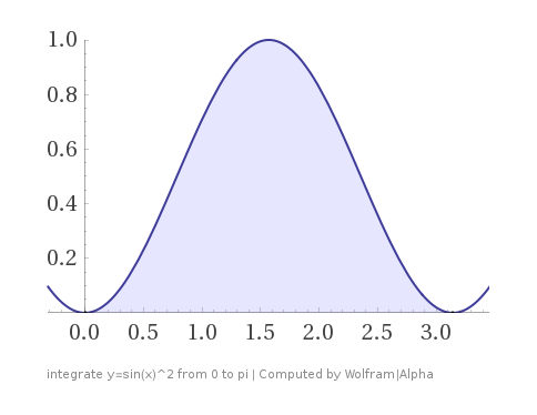
We could solve this specific problem by doing some algebra and calculus to get the exact answer analytically (which is ), but let’s pretend like we can’t, or don’t want to solve it that way.

Another way to solve this problem is to use Monte Carlo integration, which lets you solve it numerically and get an approximated answer.

How you would do that is like this:

1. Pick a random number between 0 and pi.
2. Plug that value into the function as x to get a y value.
3. Do this multiple times and take the average to get the average y value of the function.
4. Pretending that the function is a rectangle, you can use the average y as the height of the rectangle, and use pi as the width because we are looking between 0 and pi.
5. Multiply that width and height to get the area of a rectangle, which is the estimated area under the curve.

That’s all you need to do!

Monte Carlo integration is pretty powerful in how simple it is, and how it works really well even in extremely high dimensions.

As you might imagine, the more samples you take to get your average y value, the better your estimate is going to be. Unfortunately though, you have to quadruple the number of samples you have to cut the error in half, so it can take a while to get the correct answer (converge) if you need a high level of accuracy. (https://en.wikipedia.org/wiki/Monte_Carlo_method#Integration)

Here’s a C++ code snippet doing this process with 10,000 samples. Each time you run the program you’ll get a different estimate. If you take more samples, you’ll more reliably get a better answer.

double SimpleMonteCarlo()
{
    double rangeMin = 0;
    double rangeMax = 3.14159265359;

    size_t numSamples = 10000;

    std::random_device rd;
    std::mt19937 mt(rd());
    std::uniform_real_distribution<double> dist(rangeMin, rangeMax);

    double ySum = 0.0;
    for (size_t i = 1; i <= numSamples; ++i)
    {
        double x = dist(mt);
        double y = sin(x)*sin(x);
        ySum += y;
    }
    double yAverage = ySum / double(numSamples);

    double width = rangeMax - rangeMin;
    double height = yAverage;

    return width * height;
}

Below is the output of the code ran 5 times. Note that the real answer is which is 1.57079632679.

1. 1.548451
2. 1.554312
3. 1.576727
4. 1.578759
5. 1.598686

(I’m actually a bit disturbed that the 5 runs are actually sorted from low to high but whatever …)

A problem with this being based on regular old random numbers (white noise) is that sometimes the numbers will clump, giving too much weighting to one area of the function, and leave empty space where another part of the function wasn’t sampled at all.

There are many different ways to deal with this situation but two of my favorites are…

1. Blue Noise: https://blog.demofox.org/2018/01/30/what-the-heck-is-blue-noise/
2. Low discrepancy sequences: https://blog.demofox.org/2017/05/29/when-random-numbers-are-too-random-low-discrepancy-sequences/

Both of those things give more even coverage over the sampling space which means that you won’t have as large gaps of missing information from your samples.

Another way to help this is stratified sampling, where you break the sampling space up into some number of sections, and choose random numbers within each section, making sure to have samples in each of the sections. That keeps the randomness, but gives more even coverage over the sampling space.

You might be tempted to just say “If I’m taking 100 samples, i’ll just sample every 1/100th of the space evenly”. That uniform / regular sampling has some problems including aliasing, but also loses some of the positive mathematical properties that random numbers can give you (like, being able to sample from non rational numbered locations!).

A variation on stratified sampling is a technique invented by Pixar called “jittered grid” where you do even sampling, but add a small random value to each sample.

There are lots and lots of other techniques which could make up a long list of blog posts, so we’ll stop there! 🙂

More General Monte Carlo Integration

The last section was actually a simplified version of a Monte Carlo integration which was able to be simplified because it was using uniform random numbers.

Monte Carlo integration works with random numbers that have arbitrary distributions as well, not just uniform random numbers.

The process works mostly the same but there are a couple differences.

In the previous section, we got an average height and then multiplied by the width to get an estimate of the area under the curve, pretending that it was a rectangle.

The first change is to move the multiplication by the width into the loop. Instead of calculating an average height, we are instead calculating average rectangle areas.

Mathematically you get the same answer, so there’s nothing crazy there.

The second change is that instead of multiplying by the width, you divide by the probability of the number being chosen, that you plugged into the equation.

In the case of our function that we are taking samples of between 0 and pi, the probability of any single number being chosen in that range is . When we divide by that, it means we end up just multiplying by pi, so it’s mathematically equivalent to what were were doing before!

Here’s the steps for the more generalized monte carlo integration:

1. Pick a random number between 0 and pi using any random number distribution you’d like to.
2. Plug that value into the function as x to get a y value.
3. Divide that y value by the probability of having chosen that number (otherwise known as PDF(x)) to get an estimated area of the function.
4. Do this multiple times and take the average to get your result.

Here is some code to do the more general Monte Carlo integration, still using uniformly distributed random numbers.

double GeneralMonteCarlo()
{
    size_t numSamples = 10000;

    std::random_device rd;
    std::mt19937 mt(rd());
    std::uniform_real_distribution<double> dist(0.0f, 1.0f);

    auto InverseCDF = [](double x) -> double
    {
        return x * c_pi;
    };

    auto PDF = [](double x) -> double
    {
        return 1.0f / c_pi;
    };

    double estimateSum = 0.0;
    for (size_t i = 1; i <= numSamples; ++i)
    {
        double rnd = dist(mt);
        double x = InverseCDF(rnd);
        double y = sin(x)*sin(x);
        double pdf = PDF(x);
        double estimate = y / pdf;

        estimateSum += estimate;
    }
    double estimateAverage = estimateSum / double(numSamples);

    return estimateAverage;
}

Interestingly, dividing by the PDF is the same mathematically as multiplying by width in the last section – it literally ends up being a multiplication by pi (the width). The only difference is that we pulled the multiply into the loop, instead of leaving it until the end.

As an optimization, you could definitely move the divide out again (and turn it into a multiply), but I wanted to present the code as close to the core concepts as possible.

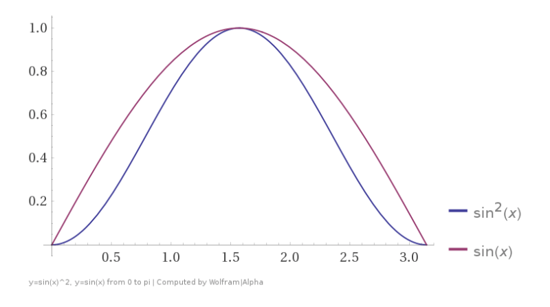
Non Uniform Random Number Distributions

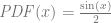
Let’s try sampling from a different random number distribution. Let’s generate random numbers which have a distribution of . You can see it compared to the function we are integrating below. They are fairly similarly shaped!

To use as a random number distribution for monte carlo integration, we’ll need to calculate the normalized PDF and we’ll also need to calculate the inverse CDF.

If you want to know more about PDFs and “whatever an inverse CDF may be”, give this a read: Generating Random Numbers From a Specific Distribution By Inverting the CDF

• The function is normalized to this PDF:
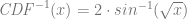
• To generate numbers from that PDF, you take a random number that is between 0 and 1 and plug it into this function, which is the inverse CDF:

Here is a code snippet doing monte carlo integration with this PDF and inverse CDF:

double ImportanceSampledMonteCarlo()
{
    size_t numSamples = 10000;

    std::random_device rd;
    std::mt19937 mt(rd());
    std::uniform_real_distribution<double> dist(0.0, 1.0);

    auto InverseCDF = [](double x) -> double
    {
        return 2.0 * asin(sqrt(x));
    };

    auto PDF = [](double x) -> double
    {
        return sin(x) / 2.0f;
    };

    double estimateSum = 0.0;
    for (size_t i = 1; i <= numSamples; ++i)
    {
        double rng = dist(mt);
        double x = InverseCDF(rng);
        double y = sin(x)*sin(x);
        double pdf = PDF(x);
        double estimate = y / pdf;

        estimateSum += estimate;
    }
    double estimateAverage = estimateSum / double(numSamples);

    return estimateAverage;
}

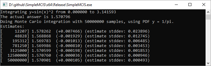
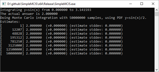
To compare this versus uniform random sampling, I'll show the progress it makes over 50,000,000 samples first using uniform random numbers, then using the shaped PDF.

Uniform aka 1/pi:

sin(x):

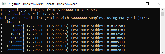
You may notice that every 4x samples, the standard deviation (which is the square root of variance) drops in half, like we talked about before. This is why path tracing takes so long. If you don’t know what path tracing is, this is why modern animated movies take so long to render.

In the results, you can see that the variance of the estimates is a lot lower using this PDF that is shaped more like the function we are trying to integrate. We got a better, more reliable answer with fewer samples. Is that pretty cool? You bet it is! When you use a PDF shaped like the function you are integrating, to get better results faster, that is called importance sampling.

Bad Random Number Distributions

If you use a PDF which is shaped very differently from the function you are trying to integrate, you will get more variance and it will take longer to converge, which is a total bummer.

Let’s try , which doesn’t look much like the function we are trying to integrate at all:

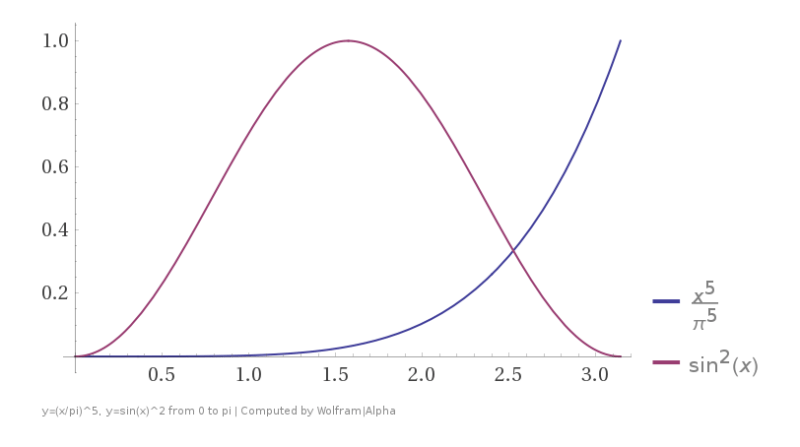
Here is the PDF and inverse CDF:

• 
• 

Here it is with 50,000,000 samples:

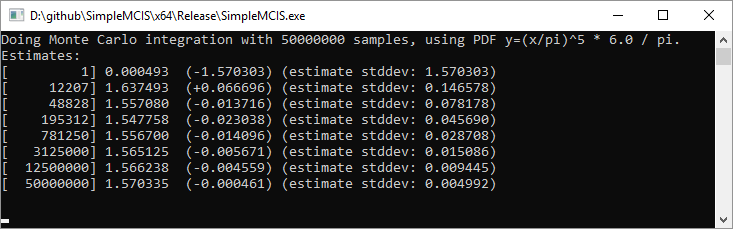
And here is the uniform sampling again as a comparison:

As you can see, it is approaching the right answer, but is taking about 10 times as long to get the same results (amount of variance) compared to uniform sampling. Ouch!

Perfect Random Number Distributions

Let’s say that we got really lucky and somehow got the PDF and inverse CDF for a function that perfectly matched the function we were trying to integrate. What would happen then?

Let’s check it out by integrating the function by using a random number distribution which has the form .

We already calculated the PDF and inverse CDF of that function earlier:

• 
• 

Here we do that with 50,000,000 samples:

WOW! As you can see, it had the right answer from the first sample, with zero variance (randomness) and it kept steady at that answer for all 50,000,000 samples.

This is a pretty neat concept, and if you know about “cosine weighted hemisphere sampling”, that does this exact thing.

Cosine weighted hemisphere samples are weighted such that you can remove the from the lighting calculations, because the random number distribution handles it for you.

It basically removes that part of randomness from the equations.

Unfortunately there are more variables and randomness in path tracing than just that term, but it helps.

Beyond this, you’d start look at other variance reduction techniques if you were interested, including multiple importance sampling.

Closing

Going into this blog post I thought “hey no sweat, i’ll make a few simple functions, calculate their PDFs, inverse CDFs and be on my way”.

I can’t believe how almost all the simple functions I tried ended up being impossible to take through the process.

for instance, you can take and solve for y to get , but if you try to solve for y, you are going to have a bad day!

I think in the future if I need to do something like this, I’d like to try fitting a curve to the (x,y) data points reordered as (y,x) data points, but there are many other methods for doing this sort of thing as well.

BTW if wondering how I was calculating std dev (aka square root of variance) while integrating, variance is “The average of the squared differences from the mean”. That means that if you know the correct answer of what you are trying to integrate, you can calculate the std dev like this:

        // Variance is "The average of the squared differences from the mean"
        double difference = integration - actualAnswer;
        double differenceSquared = difference * difference;
        averageDifferenceSquared = Lerp(averageDifferenceSquared, differenceSquared, 1.0 / double(i));
        double stdDev = sqrt(averageDifferenceSquared);

• integration is the current average estimate (if you have taken 100 samples, it’s the average of the 100 samples)
• actualAnswer is the known right answer
• averageDifferenceSquared is also the variance
• i is the number of samples you have taken, including the current one (aka start at 1, not 0)
• If you are confused about me doing a lerp to calculate an average, give this a read: Incremental Averaging

Hope you enjoyed this write up!

Anders Lindqvist (@anders_breakin) is writing up a blog post explaining monte carlo, importance sampling, and multiple importance sampling that you might be interested in if you enjoyed this. Give him a follow, and it’ll be coming out soon 🙂

Also, here is a really nice twitter thread talking about why importance sampling actually works:
https://twitter.com/Atrix256/status/1003487338633105409