The code that generated the data for this post & implements the things talked about can be found at: https://github.com/Atrix256/LDSRejectionSampling

Rejection sampling lets you convert numbers from one probability distribution into numbers from a different probability distribution. It does that by throwing numbers away.

Imagine I gave you one hundred binary digits where 50% were zeros and 50% were ones. If you wanted them to be 75% zeros and 25% ones you could throw away 33 of the ones. That would leave you with 67 numbers where 50 were zeros and 17 were ones. Now, 74.6% of the numbers are zeros, and 25.4% of the numbers are ones. The transformation worked.

That change in distribution came at a cost though, the sequence got smaller.

I previously wrote up a post about rejection sampling here:
Generating Random Numbers From a Specific Distribution With Rejection Sampling

I also wrote about inverting a CDF here, which is a more complex method where you don’t throw numbers away.
Generating Random Numbers From a Specific Distribution By Inverting the CDF

When doing rejection sampling, a random number is compared against the probability for a number to survive, and the number is thrown away if it fails that test.

This post is going to look at what happens if we use low discrepancy sequences instead of random numbers (white noise) when working with rejection sampling. We are going to try substituting LDS for the random number generation to see if we should throw away a sample, and also we are going to use an LDS to generate the sequence we use as the source of rejection sampling.

Why LDS Here?

You might be asking what the motivation is for trying low discrepancy sequences here.

As a general rule, whenever I see white noise (regular random numbers) being used, it’s usually an indication that money is being left on the table and that the situation could be improved by using something else.

My heuristic there is roughly that if it’s for graphics, with sample counts that aren’t going to converge, that blue noise is going to be a good choice to make the remaining error be least noticeable, otherwise use low discrepancy sequences.

I’ve found this to be true for almost everything I’ve tried so far.

The only two exceptions I can think of at the moment are high dimensional Monte Carlo, where white noise seems to reign supreme (not my area though so not sure. I think Sobol can go pretty high dimension??), and also in random walks.

Random walks have problems with blue noise and LDS because they are so well distributed over the sampling domain, that the random walks never really leave the origin, which isn’t useful. I believe that random walks could possibly be helped by red noise and/or high discrepancy sequences (they are a thing that exist!).

I have two other more well motivated reasons for using LDS with rejection sampling though.

Firstly, if using uniform white noise random numbers to plot a histogram, it will be a flat line, matching that flat uniform PDF, but it will only do so at the limit of an infinite number of samples. In smaller number of samples, white noise is quite lumpy. Low discrepancy sequences on the other hand will make the histogram look a lot flatter with lower sample counts (arguably blue noise does a better job at very low sample counts too). LDS will match the shape of the PDF better with fewer sample counts, but will be a better match at higher sample counts too. So, working with probabilities, being able to have better statistical properties for smaller numbers of samples seems like a no brainer.

With rejection sampling specifically, if the area of your acceptance is A, and the area you are generating random numbers in is B, the probability of acceptance of a sample is A/B. White white noise, the average acceptance rate will be right after a large number of samples, but in a lower number of samples, there may be too many rejections or too little rejections which manifests as error. Using a low discrepancy sequence instead, you should always be closer to the correct acceptance rate than white noise, which also means lower error.

Going back to our situation of having 50 ones, 50 ones and throwing away 33 of the ones… a low discrepancy sequence will mean that the ones thrown away are roughly evenly spaced in the sequence. You can see how if you threw out the first 33 ones the averages would be right for the whole sequence, but that all the ones would be at the end, with none at the beginning, which is weird. White noise can cause similar things to happen, but a low discrepancy sequence will do better at making sure the ones thrown away are more evenly spaced across the whole sequence.

The second better motivated reason is this. Imagine that whenever you accepted a sample, your function emitted a 1, and when you rejected a sample, your function emitted a 0. Let’s also say that the area you are generating random numbers in is 1, which isn’t a stretch since it’s common to generate random numbers from 0 to 1 on each axis, which defines a (hyper)cube with area 1.

If you integrate this function, the result will be A/B… the acceptance probability.

If your goal was to integrate this function, using white noise, we know we’d get the usual white noise integration situation (slow convergence, high variance, etc). You’d know to use LDS in that situation to have lower error for the same sample count compared to white noise

Rejection sampling goes through the same motions as Monte Carlo integration, it just uses the output for a different purpose.

Explanation of motivation out of the way, let’s move onto the experiments!

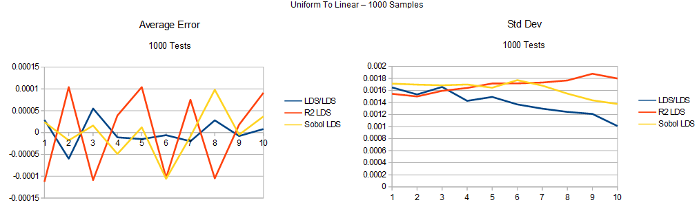
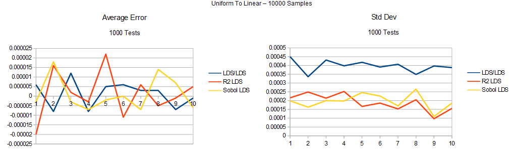
Uniform To Linear

The first test is to use rejection sampling to convert from a uniform probability distribution to a linear probability distribution.

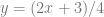
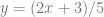
The linear PDF (Probability Density Function) is for random numbers x being between 0 and 1. Being a PDF, that function integrates to 1 over that domain of x being from 0 to 1. For the purposes of rejection sampling, we want this function to be at most 1, instead of integrating to 1, so we are going to use the probability function

We want it to be at most 1 because we are essentially wrapping the function in a box that is 1×1, rolling a 2d random number to get a point in that box, and only keeping the sample if it’s underneath our function. So, the probability function needs to fit within our box by having all values be less than or equal to 1, but we also don’t want to waste space because it would cause more numbers to be thrown away than needed, so we need to make it as large as possible by making the largest value on the function be 1.

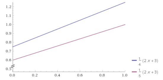
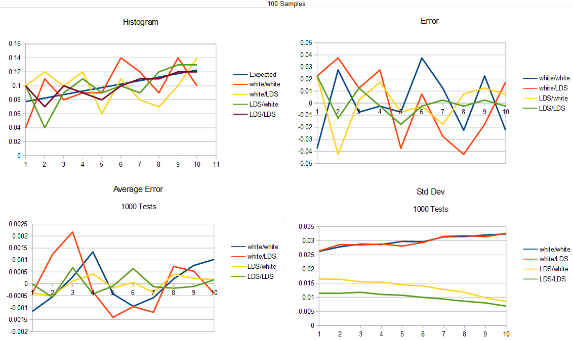
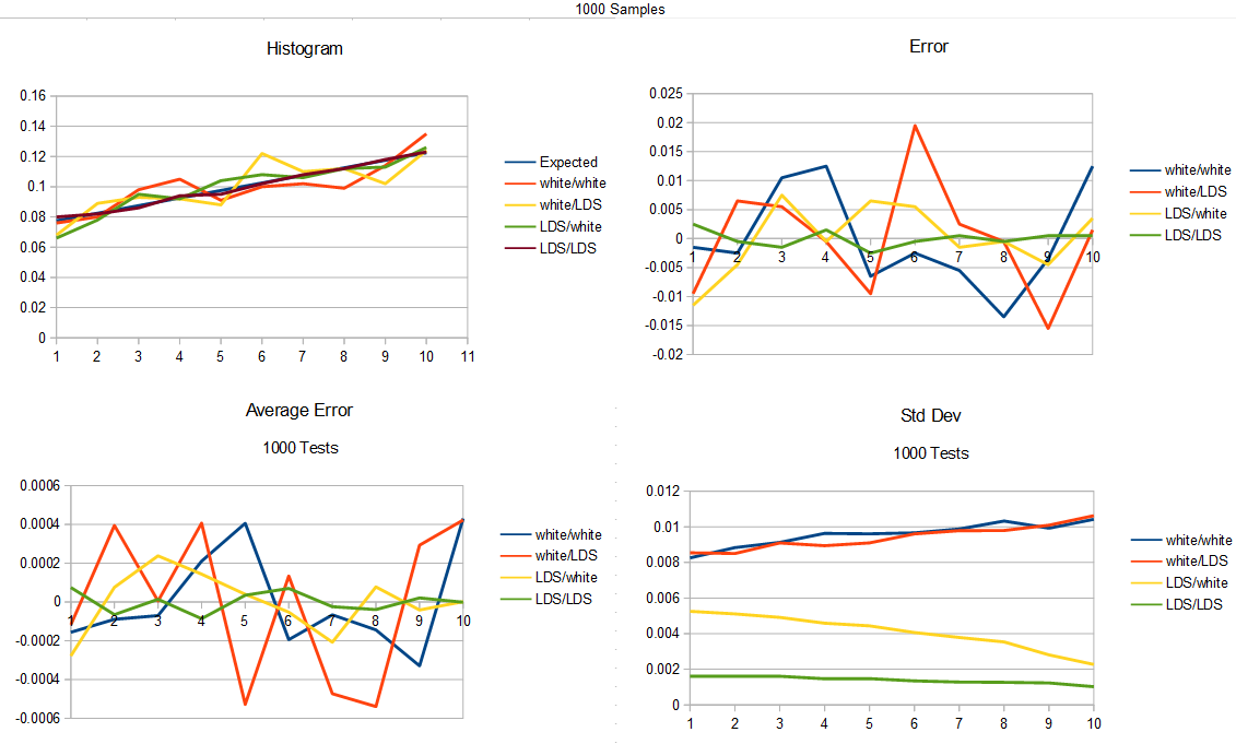
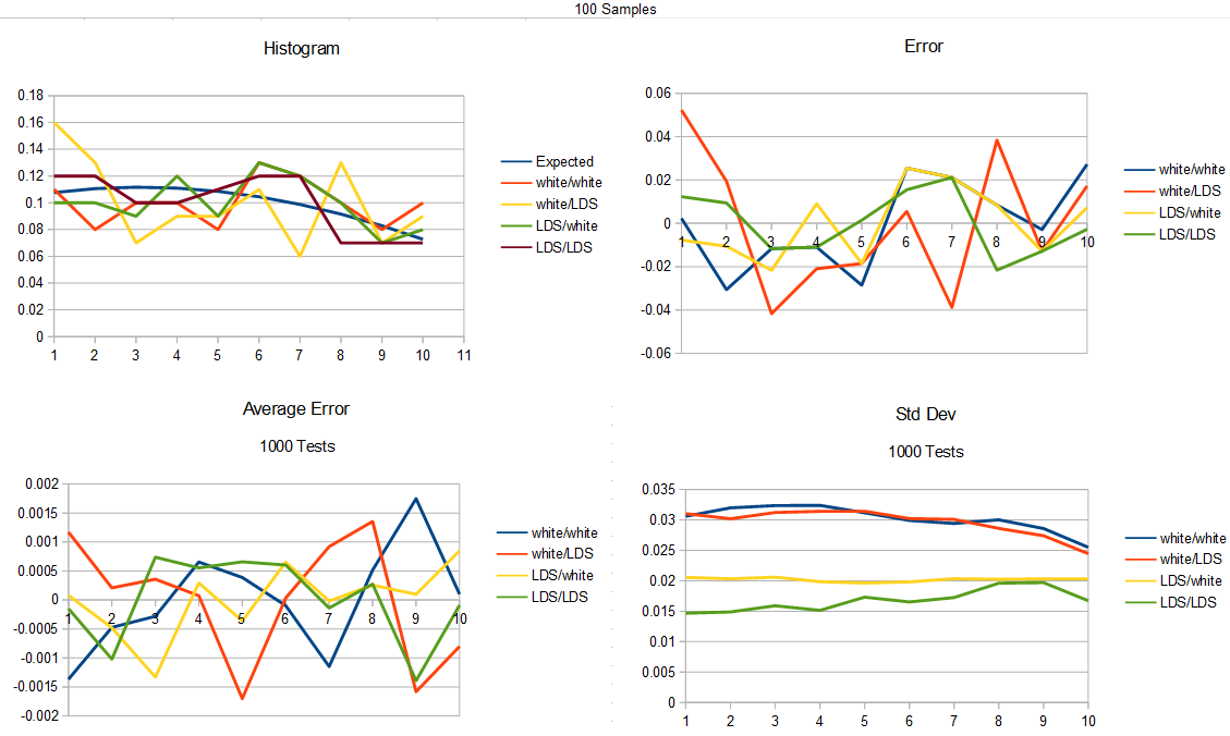
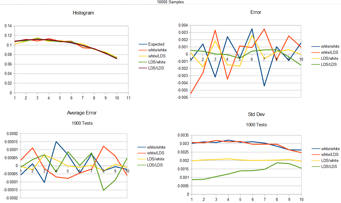
For our test, we are going to generate a number of samples in the linear distribution, by using rejection sampling on uniform distribution inputs until we have enough samples. From there we are going to break the range 0 to 1 into 10 sections and count how many numbers are in each section. That is going to give us a histogram. We are also going to subtract out the “expected” histogram value from the real PDF to show the error. We are also going to do this test 1000 times and show the average error and standard deviation.

We are going to do this for the following scenarios:

• white/white – white noise used as the input stream, white noise used to get a random number for testing against the probability of keeping the sample.
• white/LDS – white noise used as the input stream, but a LDS (golden ratio additive sequence) used to generate a “random number” for the probability test.
• LDS/white – a LDS used as the input stream (square root of 2 additive sequence), white noise used for the probability test.
• LDS/LDS – square root of 2 LDS used for the input stream, golden ratio LDS used for the probability test.

It’s also important to tell you that I’m using a (white noise) random number for the starting value of each LDS in every test. Without doing that, it would give the same results every time.

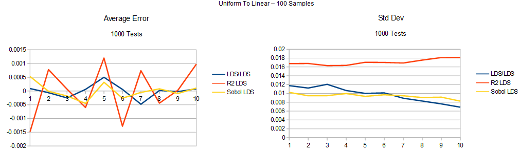
Here is the test for 100 samples generated.

Here is the test for 1000 samples generated.

Here is the test for 10000 samples generated.

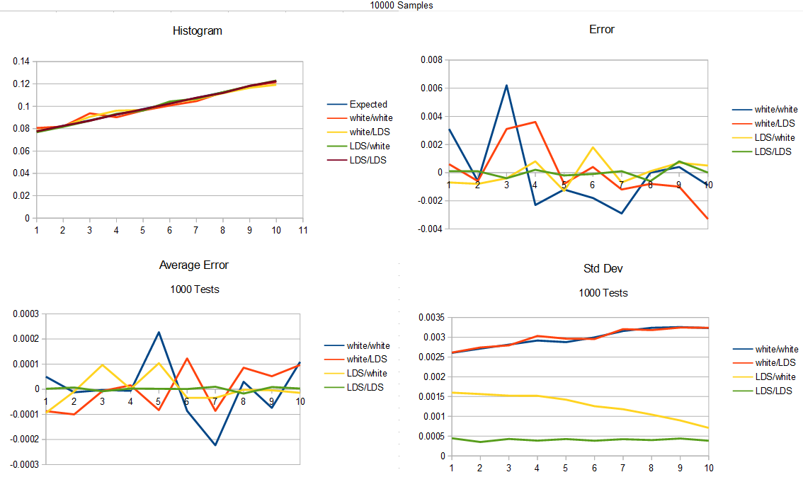
Looking at the results, it shows that the clear winner is to use a low discrepancy sequence as input to your rejection sampling, while also using a low discrepancy sequence for the probability test.

Second to that is to use a low discrepancy sequence as input, while using white noise for the probability test.

Beyond that, with white noise input, it doesn’t seem to matter much if you are using a low discrepancy sequence for the probability test or not.

That was pretty surprising when I saw that. I was sure an LDS for the probability test would be useful, and it turns out it is, but we’ll see how in a little bit.

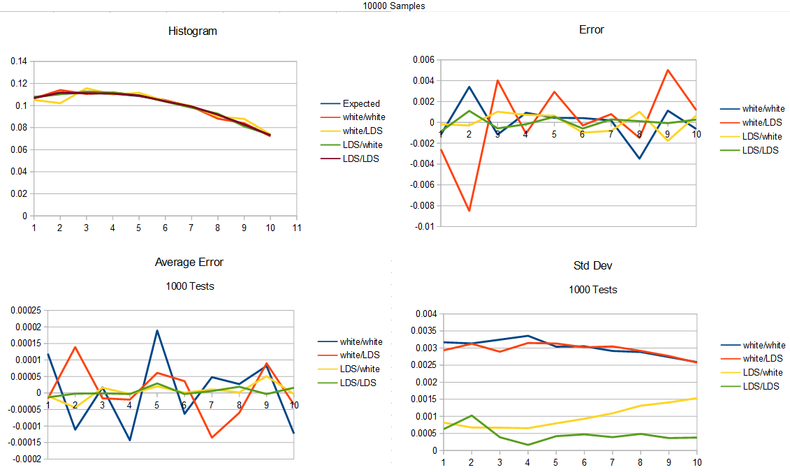
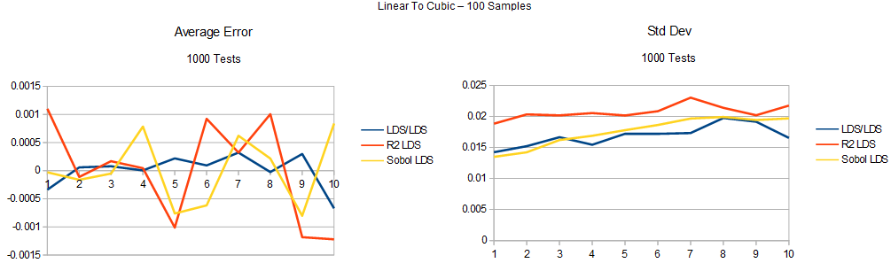
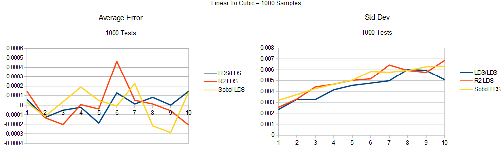
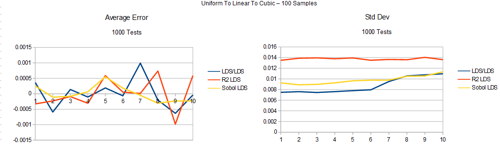
Uniform To Linear To Cubic

Let’s look at what happens if we convert a non uniform PDF to another PDF. To do that we need to generate the non uniform PDF first. An inversion method could have been used but I used rejection sampling. The type of sequence used to generate the linear PDF is the same used to convert the linear PDF to cubic.

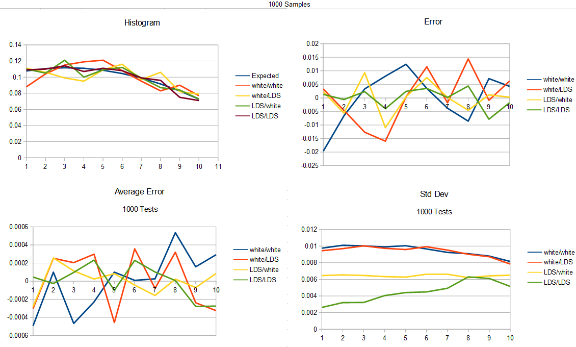
The same tests are done as before. Here is 100 samples.

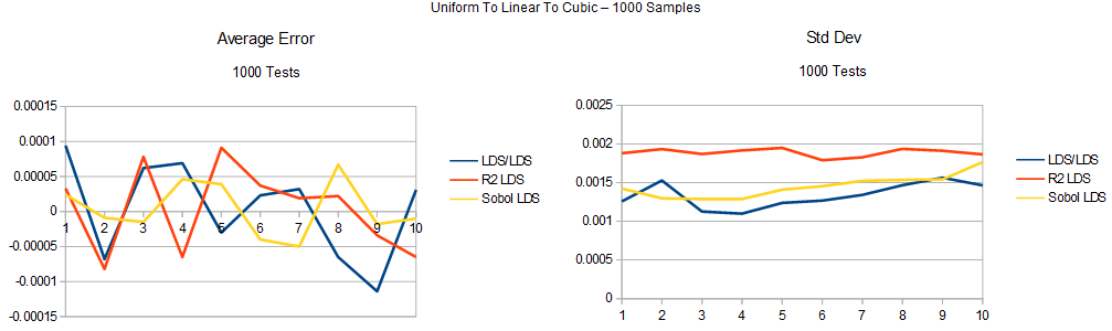
Here is 1000 samples.

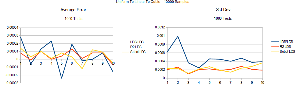
Here is 10000 samples.

We got the same results as last time basically. Low discrepancy sequence as input is better than white noise as input, and if you are using LDS as input, it’s also better to use LDS for the probability test. If you are using white noise as input, it doesn’t seem to matter if you are using white noise or LDS for the probability test.

It is interesting to see though that the standard deviation (square root of variance) of LDS/LDS is noticeably higher for the higher numbers, when it was flat going from uniform to linear in the previous section. I think that area of the curve might be sensitive to problems because it’s a really likely section in the linear pdf but less likely in the cubic pdf.

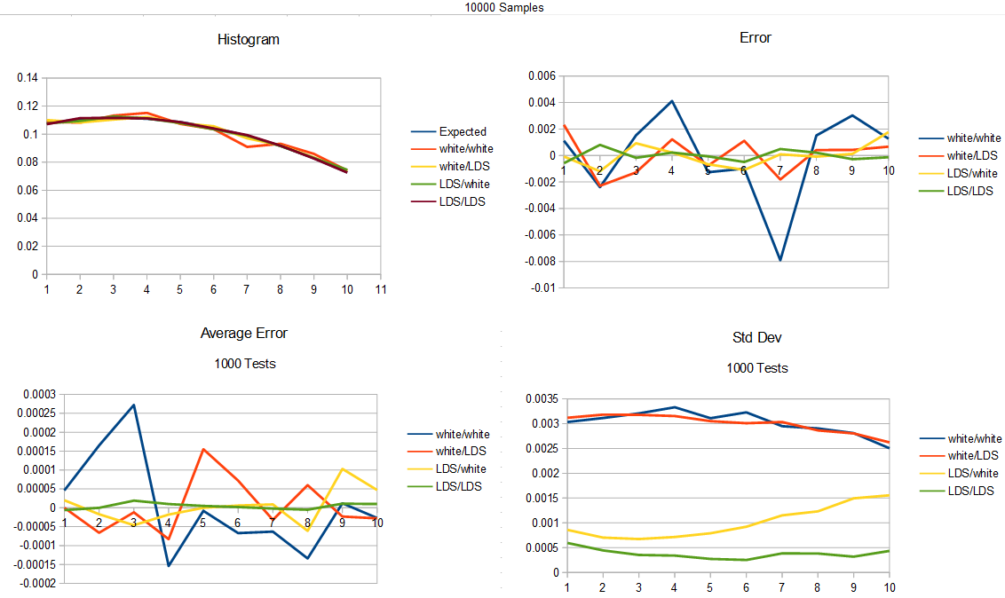
As another test, here are 10000 samples of going from uniform straight to cubic to show the difference. Now there is a noticeable spike in LDS/LDS std dev in the lower numbers, which is a bit of a mystery.

As one final test, here are 10000 samples again of going from uniform to cubic, but i swapped the roles of the golden ratio and the square root of 2 LDSs. We seemingly get better results, which isn’t too surprising if you consider that the golden ratio is a better (more irrational) number than square root 2 is, and that from our previous tests, the quality of the input sequence seems to matter more than the sequence used for the probability test.

Survival Rate

We looked at the quality of the histogram coming out of the rejection sampling, but we didn’t look at how it rejects samples.

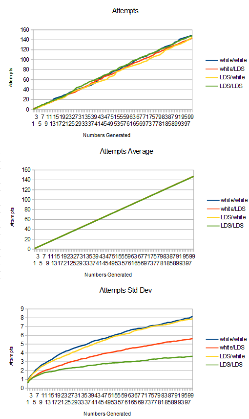
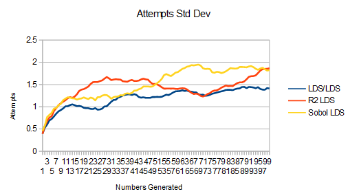
Here is the information about attempts vs samples generated from uniform to linear.

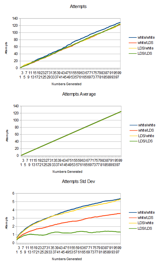
As you probably expected, LDS/LDS did best in this metric too. The main thing to pay attention to is the variance graph. Not only is the LDS/LDS variance graph lowest, it’s also flattest. This is a good thing because as we get farther to the right on the x axis, the variance of those samples sort of accumulate the variance of the samples before them too since we are looking at totals. That it’s flatter means that variance in future samples negates variance in previous samples.

Something else interesting is that in the last test where we looked at the histogram, the quality of the input mattered most to the metric we were looking at. Better quality inputs made better output histograms.

Here, the reverse is true. Better quality “random numbers” for the probability test make for better (lower) variance of sample survival.

LDS/LDS is best in both cases, but the one in 2nd place switches from LDS/white to white/LDS. 3rd and 4th place are basically tied, which is white noise and the unimportant LDS.

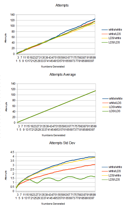
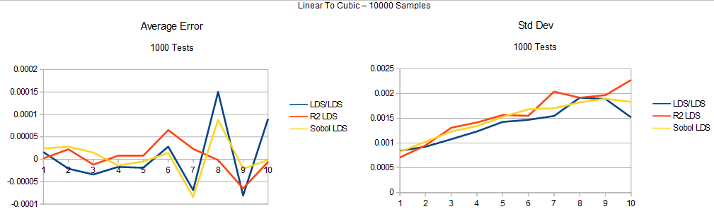
To give further proof & information, here is linear to cubic.

Here is uniform to cubic

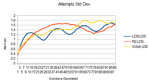
Lastly, here is uniform to cubic, but swapping the roles of golden ratio and sqrt 2 LDSs.

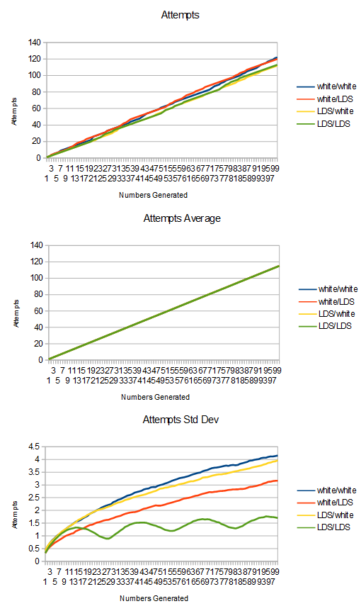
The ripples in LDS/LDS are pretty interesting. I wonder what is causing them?

Bonus: Other 2D LDS

Lefteris Stamatogiannakis (@estama2) mentioned on twitter that it might be neat to see real 2D LDS’s used for this.

The golden ratio / sqrt(2) LDS’s seem to be pretty well suited for 2d use, but they aren’t a “designed for 2D” LDS like sobol or R2 is. (R2 is by Martin Roberts, from here: http://extremelearning.com.au/unreasonable-effectiveness-of-quasirandom-sequences/)

So, I had a look! The results are mixed so I’ll let you make your own conclusions.

First, let’s look at the histogram average error / std deviation for the uniform to linear test.

Next, here is the uniform to linear to cubic test:

Here’s the uniform to cubic test. The graphs are mislabeled as uniform to linear to cubic. It’s really uniform straight to cubic. The last section goes to linear first, this one doesn’t.

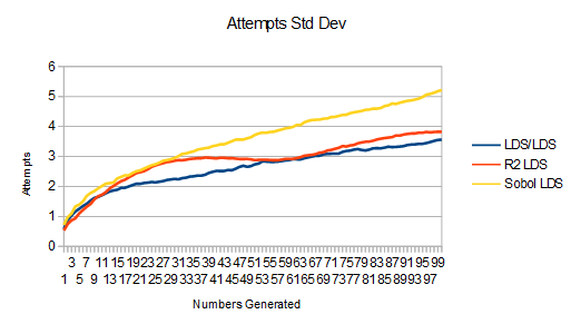
Next up are the survival graphs.

First is the uiniform to linear survival data:

Next is linear to uniform to cubic:

Last is uniform to linear to cubic: