A very cool paper was accepted to SIGGRAPH 2020 called “Monte Carlo Geometry Processing: A Grid-Free Approach to PDE-Based Methods on Volumetric Domains”

The paper is here:
https://www.cs.cmu.edu/~kmcrane/Projects/MonteCarloGeometryProcessing/index.html

You can find the authors on twitter at
@rohansawhney1
@keenanisalive.

The paper shows some really interesting things so I set out to learn more about it and arrived at the topic of this blog post.

In this blog post we are going to take common ideas of interpolation, like:

• linearly interpolating between two points on a line
• linearly interpolating between 3 points on a triangle using barycentric coordinates – or interpolating between N points on a simplex (including on a line, which is the last bullet point)
• Bilinear interpolation between 4 pixels when you zoom into a texture – or N-linear interpolation between pixels for volume textures and mipmaps

…and we are going to generalize them to interpolating data over any shape, where values are specified on the boundary of the shape (not the vertices!), and interpolated through the interior of the shape. Furthermore, the shape doesn’t even need to be contiguous, or closed.

Unfortunately, unlike the interpolation methods I mentioned above, this interpolation isn’t as friendly for real time applications.

Despite the mathy nature of the topic, I’m going to try to keep it real easy to understand, so don’t get scared off!

Introduction – Laplace’s Equation / Dirichlet problem

Let’s start with the mathy bit, in a very math light way. The below describes the mathematics of our interpolation, which is a Dirichlet problem to solve Laplace’s Equation if you wanted some terminology.

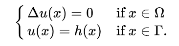
Let’s talk about it’s two parts independently:

Section #1 (The Blue Box)

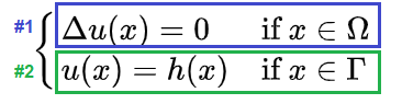
• On the left, it says “The Laplacian of the function is 0…”
• On the right, it says “…if the point is inside the shape (not on or outside the boundary)”

The Laplacian being zero inside the shape means that if you take an average of the values around any point inside the shape, they will average to the value at the center point.

If this was a 1 dimensional function, it would mean that if you pick a number on the graph, take a step to the right and the value was 1 higher than the current number, then the number if you take the same sized step to the left must be 1 lower than the current number (making sure to stay inside the boundaries). Below is a function which has a Laplacian of 0.

In 1D that means the graph is a straight line (linear) but in higher dimensions, you can get more interesting shapes. Below is a 2d function which has a Laplacian of 0.

You can see the graph here: https://www.wolframalpha.com/input/?i=z%3De%5Ex*sin%28y%29

You can see that it has a Laplacian of 0 here: https://www.wolframalpha.com/input/?i=laplacian+e%5Ex*sin%28y%29

I got that function from this great Khan Academy video: https://www.youtube.com/watch?v=JQSC0lCPG24

So, section 1 doesn’t exactly say that our function is linear, but it does give a certain smoothness to the interior that feels a bit like a linear function.

To me, I think of how a bilinear interpolation is linear on the x and y axis, but can go quadratic as soon as you get off of those axes. Having a Laplacian of zero seems to satisfy the spirit of that “linear on an axis” property, without being limited to a specific axis.

Section #2 (The Green Box)

• On the left it says “The function has specific values…”
• On the right it says “…if the point is on the border”

All this means is that there are values along the border, and it doesn’t matter how those values are defined.

Putting it Together

So section 2 says there are values on the border of the shape, and section 1 says that any point inside the shape is an average of the values around it – even if that point is near the border. This defines how our interpolation works.

So, let’s take a walk. Pretend you started at a border and walked across the shape in a straight line until you hit the border at the other side of the shape.

When you started walking, you’d have the value of the border where you started. As you walked into the shape, the value would mix with values from other nearby borders (basically weighted by their distance to you).

When you hit the midway point of your walk, the border you started at and the border you ended at would have equal weighting in the current value you had, but other border values would be contributing as well.

When you got closer to the border you are ending at, the value there would start to weigh more heavily into the value, until you finally reached the destination point of your walk, and the value was just the border value there.

This essentially is our interpolation, as described by those two mathematical statements.

How To Do It – Walk On Spheres Algorithm

If you have ray marched signed distance fields, prepare to have your mind blown. There is a huge similarity here 🙂

To interpolate data in a shape, where the data values are defined by values at the boundary, you need to be able to get a distance from a point to the nearest border. You don’t need to be able to get a direction, just the distance. You need a (signed) distance field.

If you can’t get an ACTUAL distance to the border, but can get a conservative estimate (an estimate that is guaranteed to be <= the actual distance), that works fine too.

Here is a neat article from Inigo Quilez that talks about how to get that kind of an estimate using function gradients: https://www.iquilezles.org/www/articles/distance/distance.htm

So the algorithm is to start at your point and…

1. Get the distance from the point to the border. This defines a sphere representing the largest step you can take without leaving the shape. (sphere if 3d, circle if 2d, hypersphere if 4d or higher, line segment if 1d)
2. If the distance to the border is smaller than some epsilon, return the value at the border there.
3. Else, take a step of that distance in a uniform random direction
4. GOTO 1

If you do that full loop 1 time, you will get a single value. This is 1 sample.

If you do that N times and average the result, you’ll get a value that approaches the correct value. This is where the “monte carlo” part mentioned in the paper comes in. We are doing monte carlo integration, where each sample is a random walk in the shape from the starting point to whatever part of the border it exits at.

Higher values of N give more accurate results with less error.

That is all there is to it!

It works because the likelihood of hitting an specific boundary point depends entirely on how far it is from your starting point. Closer boundary points are more likely to be reached, while farther boundary points are less likely to be reached.

If you are doing this process for an image, you would run this N times for each pixel individually, to get a noisy result that got less noisy as you took more samples, just like path tracing. You could even use denoising on the image before it converged.

A non obvious detail is that the shape doesn’t need to be convex. It can be concave which means that the random walk needs to “go around corners” to reach borders. The distance used for interpolation weighting is the “around the corner” distance, not a straight line distance where the straight line exits the shape and then re-enters it.

Another interesting thing is that the shape doesn’t strictly need to be closed. You could have a U shape with values along the U, and this algorithm works just fine. It just now applies to shapes inside of the bowl of the U as well as the points outside the bowl of the U, off into infinity. (Is this still interpolation? it isn’t quite extrapolation I don’t think… hrm!)

You could also have multiple shapes that aren’t connected scattered around with values on them and this algorithm still works just fine.

Being Monte Carlo integration, you can apply ideas like importance sampling, and Russian Roulette too. Importance sampling to reach boundaries more quickly. Russian Roulette to kill paths that are wandering away form useful areas in an unbiased way.

I haven’t found a way to apply low discrepancy sequences for faster convergence though, nor have I found a way to apply blue noise for better perceptual error. The search continues though and there are some resources regarding LDS in the links section.

Examples – My Shadertoys

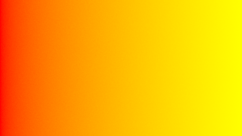
I wrote a shadertoy which uses this technique to do 1d interpolation from red to yellow. You could do the same thing with a lerp easily, but it is a simple demonstration of the technique.

The shadertoy is at https://www.shadertoy.com/view/ttByDw

Here it is after 1 sample. Every pixel has done one random walk on a numberline.

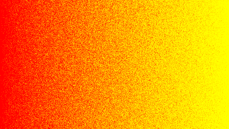
Here it is after 10 seconds, which is 600 samples, because of vsync locking it to 60fps.

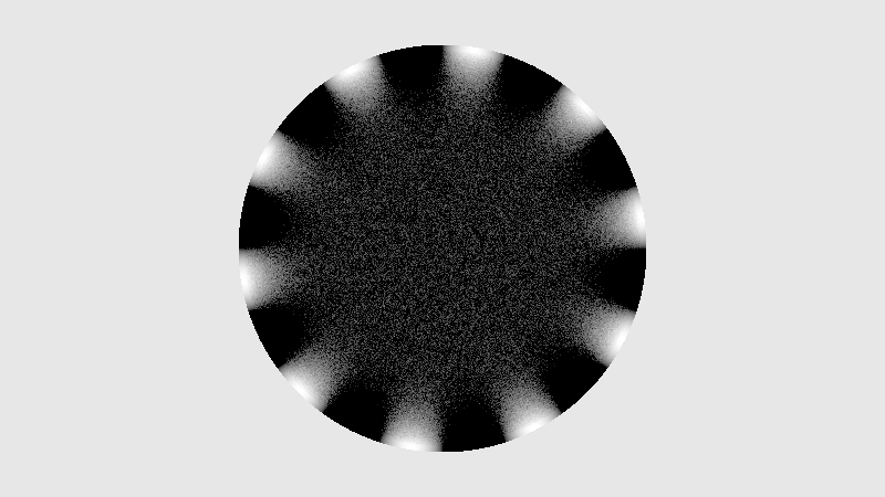
I also made a shadertoy which works in 2D using 2D SDFs, with a handful of scenes (there is a SCENE define in the common tab to control which is being viewed) at https://www.shadertoy.com/view/wtSyWm

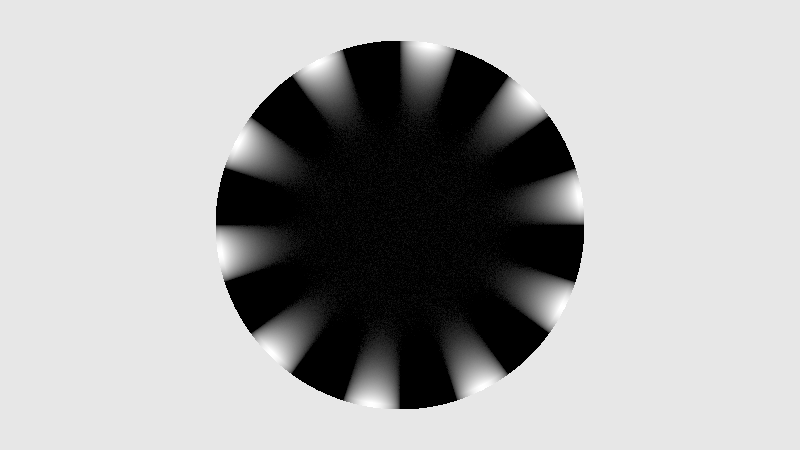
From that shadertoy, here is a circle which uses a sine wave around the border to make sections of white and black. This is the noisy unconverged version.

Here it is more converged.

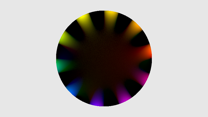
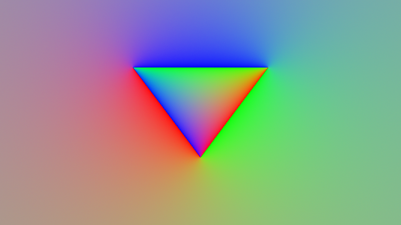
Here is a version using rainbow colors around the border:

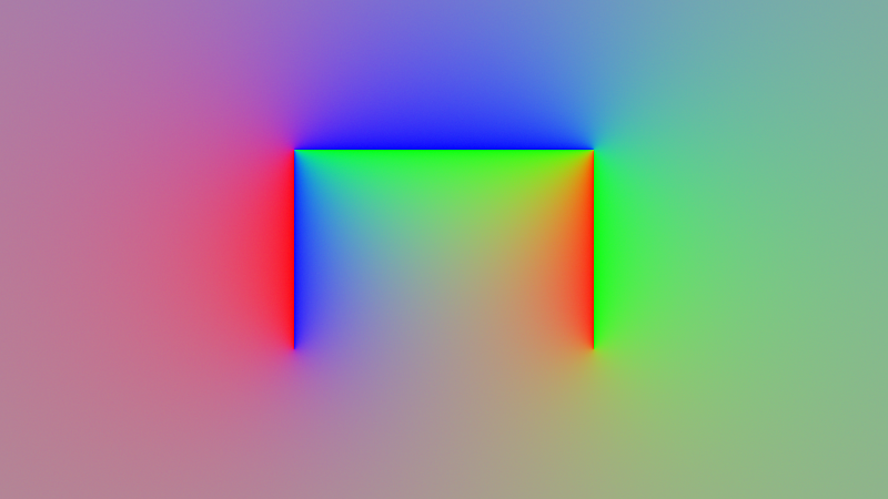
Here is a setup using 3 lines to make a triangle, where each line has a different color on the inside and the outside. Even though the lines are boundaries, there is an “inside and outside”, so the boundary isn’t a typical boundary.

Here is the same setup, but opening the triangle into a U shape, to show it works with shapes that aren’t closed.

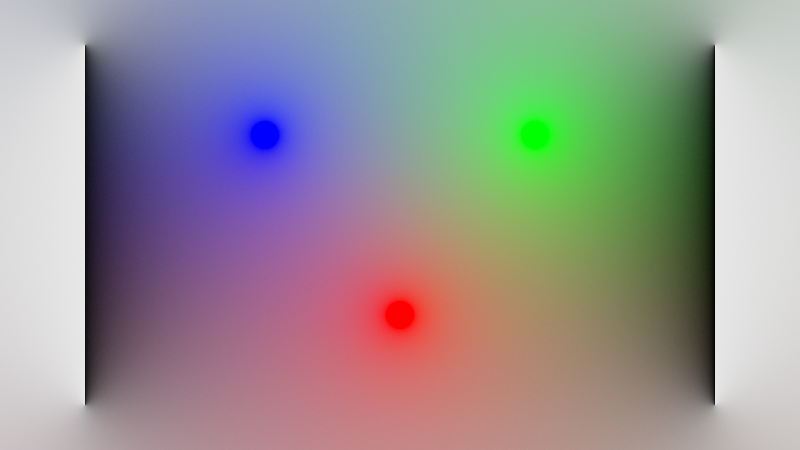
Here are 3 circles and two lines. The lines are black colored on the side facing the center of the screen, and white colored on the outside.

A 3d version will be shown in the next section!

Examples – Other Shadertoys

The website for the paper on monte carlo geometry processing links to 3 really interesting shadertoys. I want to explain what they are doing real quick, because it is pretty clever stuff.

The first is by inigo quilez (@iquilezles). https://www.shadertoy.com/view/WsXBzl

This shadertoy does the same things my 2d shadertoys were doing. There are two lines that cross each other, and have a different color on each side.

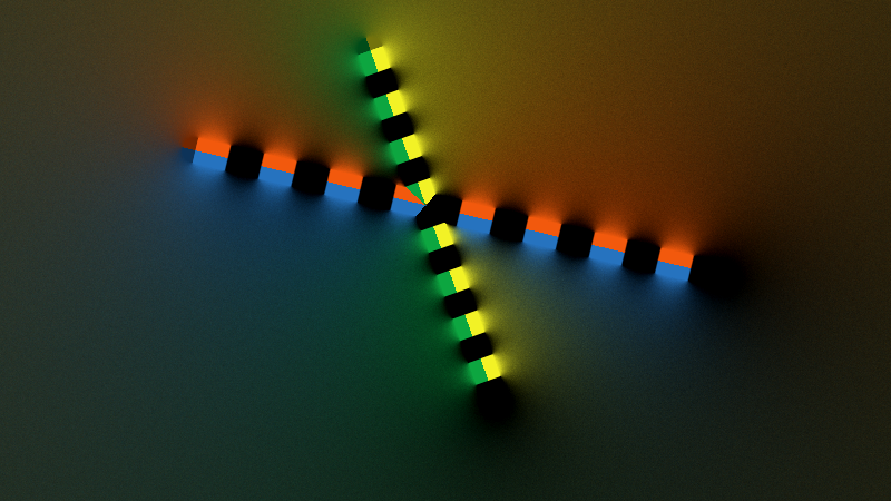
The next is also by inigo. https://www.shadertoy.com/view/WdXfzl

Believe it or not, this is also doing the same thing as the last shadertoy, and my 2d shadertoy. It’s just interpolating colors between lines. Below is the lines without the interpolation/diffusion!

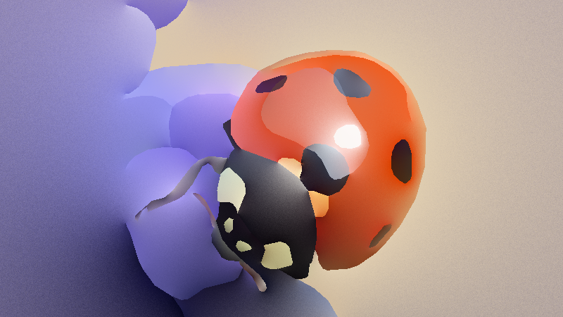
The last shadertoy is by Ricky Reusser (@rickyreusser). https://www.shadertoy.com/view/wdffWj

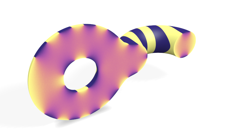
This one is actually doing the algorithm in 3d. if you are looking at the outside of the shape, those yellow/black zebra stripes are the boundary conditions. The pickish color in the middle is the interpolated values, but they are tinted slightly red, as a variation on the plain vanilla algorithm.

Closing

So, in this blog post we talked about how to use monte carlo integration and the walk on spheres algorithm to interpolate data between very arbitrary borders in any dimension.

This is a large part of the basis of the paper on monte carlo geometry processing, but it goes a lot farther than this as well. I don’t really understand how the other things shown in the paper use WOS to do what they do. As I learn more, I may make more shadertoys and make other blog posts.

Links

Since (signed) distance functions are really important to this technique, you might be wondering where you can go to read more about them. Luckily inigo quilez has you covered, and has been writing stuff about them for years. He talks about them in the context of ray marching, but that is an extemely similar usage case. Basically just imagine that instead of a random direction walk, you walked a specific direction down a ray, from the ray origin, to see what the ray hit. That is ray marching in a nutshell.

Here is information from him about 2d distance functions:
https://www.iquilezles.org/www/articles/distfunctions2d/distfunctions2d.htm

Here is information about 3d distance functions:
https://www.iquilezles.org/www/articles/distfunctions/distfunctions.htm

Here is another write up on this topic
“Walk on Spheres Method in Julia” from Philip Zucker (@SandMouth)
https://www.philipzucker.com/walk-on-spheres-method-in-julia/

Apparently harmonic coordinates are related, and seem to be a generalization of barycentric coordinates.
“Harmonic Coordinates for Character Articulation” from Pixar
https://graphics.pixar.com/library/HarmonicCoordinatesB/paper.pdf

I believe these techniques can be applied to Poisson blending, where you paste pixel deltas (instead of absolute values) into a destination image, so that what you are pasting takes on the lighting and coloring of the destination image.
https://erkaman.github.io/posts/poisson_blending.html

Poisson blending and others are talked about in this next paper. WoS can solve the Laplacian equation, but it can also solve a generalization of the Laplacian equation called the Poisson equation, so Poisson is very related.
“Poisson Image Editing”

Click to access 2003_siggraph_perez.pdf

“Walk on Spheres Method” on wikipedia
https://en.wikipedia.org/wiki/Walk-on-spheres_method

Regarding trying to apply low discrepancy sequences (or blue noise!) to the random walk on spheres, here is some interesting info about quasi random (aka LDS) random walks.
https://hpi.de/friedrich/research/rotor-router/theory.html

Thanks for reading!