When running PCA (Principle Component Analysis) on a data set, it gives back a set of orthogonal axes for that data, as well scalar values telling you the importance of each axis.

When sorting the axes by importance, the first axis is the axis that has the most variation of the data, so is the best approximation of the data with a straight line. The second axis is perpendicular and is the axis that adds the most variation of the error from the first line. The third axis is perpendicular and adds on the most remaining variation, same with the fourth, fifth and so on, up to the dimensionality of your data set.

While you can transform your data to use these axes and reconstruct the data perfectly, PCA is useful because you can decide to throw away some number of the least important axes, thus reducing the dimensionality of the data!

That can be useful for data analysis (reasoning about 2D data is a lot easier than 4D data!), but it can also be a form of data compression, if the error introduced by throwing away one or more dimensions is acceptable.

PCA itself is pretty easy to explain, but to implement it yourself, you need to be able to calculate the eigen values and eigen vectors of a matrix. Those operations are notoriously difficult to do in robust ways, so the common wisdom is to not implement them yourself, but to use software like python or libraries like Eigen (https://eigen.tuxfamily.org/) to do the hard bits for you.

To crack open the black box a bit though, I implemented it in plain C++. It’s about 800 lines including comments, generated all the data in this blog post, and you can check it out here: https://github.com/Atrix256/PCA.

Calculating PCA

To calculate PCA you…

1. Center the data
2. Calculate the covariance matrix
3. Calculate the covariance eigen values and eigen vectors
4. Transform the data
5. Recover the data

Let’s go through this step by step.

1. Center the Data

For this you just calculate the average of your data and subtract the average from all data points.

This makes the data centered on the origin which is important for PCA since it is meant to find the axes of importance in the data – NOT fit a line to the data.

Later on if you want to recover your uncentered data from the PCA encoded data, you’ll need to keep this average around to add it back in. Something to keep in mind if thinking about using PCA for data compression.

2. Calculate the Covariance Matrix

If you have N dimensional data, the covariance matrix will be NxN.

Each cell of the covariance matrix i,j will contain the covariance value between all the data in dimension i and dimension j. Since the covariance of a variable with itself is the variance, the diagonal of the matrix will have the variance values of the dimensions.

As a recap, covariance is calculated as:

Variance is just covariance of a value with itself, so is calculated as:

If your data represents a sample of the data instead of the entire data, you’ll need to use sample variance instead, which divides the sums by (n-1) instead of dividing by n.

3. Calculate the Covariance Eigen Values and Eigen Vectors

This is the part that is less easy, where we calculate the eigen values and eigen vectors of the covariance matrix. The eigen vectors are the axes of importance we mentioned before, and the eigen values are how important each one is.

First we need to calculate the eigen values.

I calculate them using the “QR Algorithm” (https://en.wikipedia.org/wiki/QR_algorithm) which is an algorithm that gives you approximate eigen values. It works by repeatedly doing QR decomposition (https://en.wikipedia.org/wiki/QR_decomposition) on the matrix and setting the matrix to R*Q for the next iteration. You do this process until a certain number of iterations has occurred, or all non diagonal elements of the matrix are close enough to zero for your liking. When finished, the approximate eigen values are the diagonal values of the matrix.

I loop until the largest non diagonal value is less than 0.0001, but didn’t play around with this very much. You can see this code at https://github.com/Atrix256/PCA/blob/main/vecmath.h#L321.

As part of the QR decomposition, I use the Gram-Schmidt process (https://en.wikipedia.org/wiki/Gram%E2%80%93Schmidt_process) to make orthogonal vectors.

There are other ways to get eigen values, and other choices you can make in the QR algorithm. I didn’t implement shifting, which helps convergence, and I’ve heard that Householder reflections are much better quality, and not that much more difficult to implement.

In any case, this works well enough for me to get good enough eigen values in my test cases.

Now that we have the eigen values, we need to get the eigen vector associated with each one. To do that, I use the inverse iteration algorithm (https://en.wikipedia.org/wiki/Inverse_iteration) which gives you an eigenvector associated with an approximate eigen value. It’s a pretty simple algorithm that just inverts a matrix and then repeatedly puts a randomly initialized vector through it. I do that for 10,000 iterations. The code for it is at https://github.com/Atrix256/PCA/blob/main/vecmath.h#L398.

I also normalize the eigen vectors and re-calculate the eigen values from the newly found eigen vectors to make them match up better. I had to switch from floats to doubles at one point as well, but may have just been doing something silly, like letting numbers get too small without clamping them to zero.

4. Transform the data

Sorting the eigen vectors from largest to smallest, you can then make them be columns of a matrix. This is the matrix you use to convert your data into “PCA space”. To reduce dimensionality you can either throw away columns from the right at this point, or you can wait until after transforming the data into the new space. It’s up to you to decide how many columns you can get away with throwing away for your usage case.

5. Recover the Data

To recover your data from “PCA space”, you make the eigenvectors for the dimensions that you didn’t throw out as rows in a matrix instead of columns. Multiply the PCA data by this matrix to get the data back minus the information contained in the lost columns.

Not too bad right? I want to re-iterate that while this code works for my handful of test cases on this blog post, it almost certainly is not production ready. It’s just a semi naive implementation for learning purposes.

Result: Gaussian Blur Kernel

First let’s PCA a 3×3 gaussian blur kernel with a sigma of 0.3.

The filter itself is:

[0.002300, 0.043200, 0.002300]
[0.043200, 0.818000, 0.043200]
[0.002300, 0.043200, 0.002300]

The eigen values and eigen vectors are:

[0.134147] [0.052641, 0.997225, 0.052641]
[0.000000] [0.000000, 0.000000, 0.000000]
[0.000000] [0.000000, 0.000000, 0.000000]

Interestingly, you can see that there’s only one non zero eigenvalue. That means that our data is in fact a rank 1 matrix in disguise! In other words, all the rows are just scalar multiples of each other. We could then replace each row with a single scalar value to multiply the eigen vector by which would reduce our data from 3D to 1D and 1/3 the storage size!

The two rows of zero eigen values is due to the fact that gaussian blurs are separable, so rows (or columns) really are just scalar multiples of each other. This test was inspired by a post from Bart Wronski on how to use SVD to separate non separable filters: https://bartwronski.com/2020/02/03/separate-your-filters-svd-and-low-rank-approximation-of-image-filters/

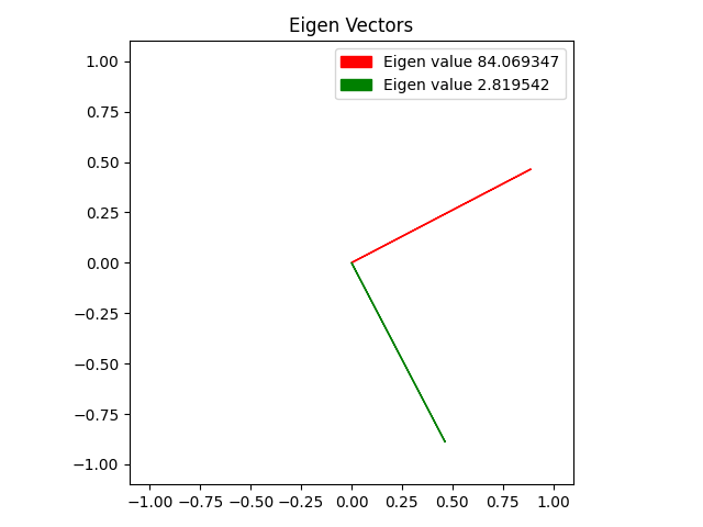
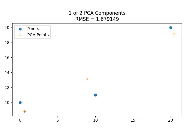
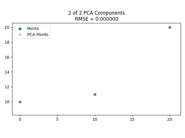
Result: 2D Data

Here’s the eigenvectors of some 2D data, then showing it reduced to 1 dimension along the larger eigenvector, then showing it including the smaller eigenvector, which makes it fit the data perfectly.

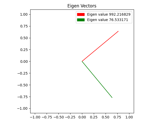
Here is the same with some different data points.

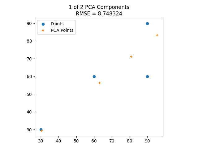
Result: 3D Data

I took some 3D data from a page that was real helpful when trying to understand PCA better (https://towardsdatascience.com/the-mathematics-behind-principal-component-analysis-fff2d7f4b643):

[90.000000, 60.000000, 90.000000]
[90.000000, 90.000000, 30.000000]
[60.000000, 60.000000, 60.000000]
[60.000000, 60.000000, 90.000000]
[30.000000, 30.000000, 30.000000]

The eigen values and eigen vectors are:

[910.069953] [0.655802, 0.429198, 0.621058]
[629.110387] [0.385999, 0.516366, -0.764441]
[44.819660] [0.648790, -0.741050, -0.172964]

And here is the RMSE for the data when PCA’d to different numbers of dimensions:

[1] 25.960163
[2] 6.694749
[3] 0.000000

At 1 component the data is:

[88.540569, 74.751951, 81.346364]
[72.547174, 64.284878, 66.200303]
[63.419540, 58.311187, 57.556254]
[75.638271, 66.307884, 69.127633]
[29.854445, 36.344100, 25.769445]

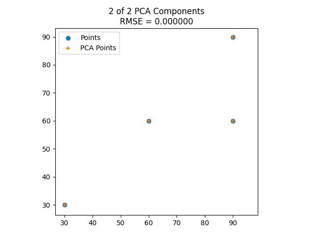
At 2 components:

[83.264247, 67.693599, 91.795721]
[90.954764, 88.909466, 29.745464]
[62.525570, 57.115286, 59.326695]
[65.892097, 53.270028, 88.429194]
[27.363322, 33.011622, 30.702926]

At 3 components, it matches, since no dimensionality reduction occured.

[90.000000, 60.000000, 90.000000]
[90.000000, 90.000000, 30.000000]
[60.000000, 60.000000, 60.000000]
[60.000000, 60.000000, 90.000000]
[30.000000, 30.000000, 30.000000]

Closing and Links

When you fit PCA to data, it minimizes the distance from the data point to the fit line. This is in contrast to least squares which only minimizes the distance on the y axis. One reason I wanted to dive deep into PCA was to see if it could be used to fit piecewise non linear curves like least squares can. After learning more, that seems to be swimming against the current for PCA, which is more aimed at things like making 3d vectors be storable as 2d vectors. I’ll bet what I was thinking of is possible, but I couldn’t really find info on it. I did find out that “Total Least Squares” exists which does the same kind of fitting though, so I think I should look more into that. Also “non linear dimensional reduction” is a topic as well.

It turns out too that a better way to do PCA than what I’ve done above is to use SVD to do PCA. I plan on doing a post on SVD soon and should be able to talk more about that then.

These two links were super helpful while writing this code:
https://towardsdatascience.com/the-mathematics-behind-principal-component-analysis-fff2d7f4b643
https://towardsdatascience.com/principal-component-analysis-explained-d404c34d76e7

Since rolling your own PCA is usually frowned on due to the numerical complexity of things involved, here’s some info about how to do PCA in python (also, in C++ you might want to use that Eigen library i mentioned before)
https://stats.stackexchange.com/questions/235882/pca-in-numpy-and-sklearn-produces-different-results

Check out this link for a neat usage case of PCA for texture compression on textures used in PBR (Physically Based Rendering):
https://bartwronski.com/2020/05/21/dimensionality-reduction-for-image-and-texture-set-compression/