The last post (https://blog.demofox.org/2022/07/10/programming-pca-from-scratch-in-c/) talked about calculating PCA from scratch, and gave some C++ code which did just that.

The post mentioned that the code was somewhat naïve and shouldn’t be used in situations that matter, because the operations done for PCA were notoriously complex numerically and difficult to make robust. It said that a library called Eigen should be used if doing things like that in C++. This post does just that – it uses the Eigen library to compute SVD (Singular Value Decomposition), and also shows how to calculate PCA from SVD, which is a more robust way of doing it than I showed in the last post. Specifically, PCA from SVD doesn’t need to calculate the covariance matrix, which can be a source of numerical problems.

SVD is pretty closely related to PCA, with the main differences being that the formula is different, and data doesn’t need to be centered for SVD, while it does for PCA.

The 190 lines of C++ code that goes along with this post is at https://github.com/Atrix256/SVD. The code uses the Eigen library, which is a header only library.

Calculating SVD

This video does a great job of explaining how to calculate SVD. Feel free to give it a watch, but i’ll also explain below. https://www.youtube.com/watch?v=cOUTpqlX-Xs.

SVD takes as input a matrix () sized MxN (it doesn’t have to be square) and breaks it apart into a rotation (), a scale (), and another rotation (). Any matrix can be decomposed this way:

The scaling matrix has zeros everywhere except the diagonal. The values on the diagonal are called the “Singular Values” and they also describe how “important” each row of and column of is. Just like PCA, you can get rid of the ones with the lowest singular values and thus reduce dimensionality of the data. This is called “Truncated SVD”.

So how do you calculate SVD?

First you multiply your (possibly rectangular) matrix with to make the square matrix .

The eigenvectors of get put together as column vectors to make the matrix .

The matrix has the square roots of the eigenvalues of along the diagonal.

The matrix is made by multiplying and normalizing the columns.

That’s all there is to it!

C++ Code

Using eigen to calculate SVD as described above is pretty straightforward:

Matrix2d C;
C <<
    5.0f, 5.0f,
    -1.0f, 7.0f;

// Calculate SVD as described in https://www.youtube.com/watch?v=cOUTpqlX-Xs
{
    Matrix2d CTC = C.transpose() * C;

    EigenSolver<Matrix2d> es(CTC);
    EigenSolver<Matrix2d>::EigenvalueType eigenValues = es.eigenvalues();
    EigenSolver<Matrix2d>::EigenvectorsType eigenVectors = es.eigenvectors();

    auto V = eigenVectors;

    MatrixXcd sigma;
    {
        sigma = MatrixXcd::Zero(eigenValues.rows(), eigenValues.rows());
        for (int i = 0; i < eigenValues.rows(); ++i)
            sigma(i, i) = sqrt(eigenValues[i].real());
    }

    MatrixXcd U = C * V;
    for (int i = 0; i < U.cols(); ++i)
        U.col(i).normalize();

    cout << "C = \n" << C << "\n\n";

    cout << "U = \n" << U.real() << "\n\n";
    cout << "sigma = \n" << sigma.real() << "\n\n";
    cout << "V = \n" << V.real() << "\n\n";

    cout << "U * sigma * VT = \n" << (U * sigma * V.transpose()).real() << "\n\n";
}

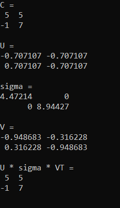
Running that gives this output. The final output of U*sigma*VT shows that putting the decomposed matrices back together gives you the original data.

While the Eigen library has interfaces to let you calculate eigenvalues and eigenvectors, it also has higher level functionality – including performing SVD itself! There are two ways to do SVD in Eigen… one is better for smaller matrices (JacobiSVD), the other is better for bigger matrices (BDCSVD). In this case, I use the one better for bigger matrices, because AFAIK it’s fine for smaller ones too, just a bit slower.

Matrix2d C;
C <<
	5.0f, 5.0f,
	-1.0f, 7.0f;

// Calculate SVD using the built in functionality
{
    BDCSVD<Matrix2d> svd(C, ComputeFullU | ComputeFullV);

    auto U = svd.matrixU();
    auto V = svd.matrixV();
    auto sigma = svd.singularValues().asDiagonal().toDenseMatrix();

    cout << "C = \n" << C << "\n\n";

    cout << "U = \n" << U << "\n\n";
    cout << "sigma = \n" << sigma << "\n\n";
    cout << "V = \n" << V << "\n\n";

    cout << "U * sigma * VT = \n" << U * sigma * V.transpose() << "\n\n";
}

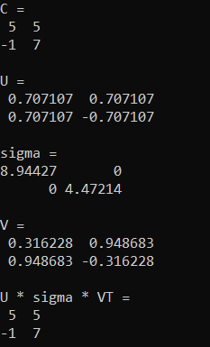
Running that outputs this, which is the same as before, except the eigenvalues are switched, and one of the eigenvectors was multiplied by -1 (opposite magnitude but still the same eigenvector).

Calculating PCA With SVD

To calculate PCA using SVD, all you need to do is run SVD and then multiply C with V. Here’s some code where we use the 3×3 Gaussian kernel with sigma 0.3 from last blog post, and run PCA on it again.

// PCA!
{
    Matrix3d newC;
    newC <<
        0.002300, 0.043200, 0.002300,
        0.043200, 0.818000, 0.043200,
        0.002300, 0.043200, 0.002300;

    BDCSVD<Matrix3d> svd(newC, ComputeFullU | ComputeFullV);

    auto U = svd.matrixU();
    auto V = svd.matrixV();
    auto sigma = svd.singularValues().asDiagonal().toDenseMatrix();

    cout << "C = \n" << C << "\n\n";

    cout << "V = \n" << V << "\n\n";

    cout << "sigma = \n" << sigma << "\n\n";

    cout << "C * V = \n" << newC * V << "\n\n";

    cout << "Principle Direction = \n" << (newC * V).col(0).normalized() << "\n\n";
}

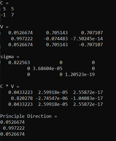
When we do that we get this. The sigma tells us that there is basically only one non zero component (the others are close enough to zero to be considered zero) and the principle direction matches what we found in the last post as well. Looks like it’s working!

SVD Of Image

Next up, we’ll take an image with size WxH, make a matrix that is Wx(3H) in size, and perform truncated SVD on it, with different numbers of singular values. The matrix is 3 times as tall because we are going to separate each row of RGB pixels into three rows of pixels; one row for each color channel. The code to do this is in the github repo, so go have a look and play around with it if you want to 🙂

First is the old man from legend of zelda 1 in NES. First is the original image, then 1 singular value, then 5%, 10%, 15%, 20%, 25% and 50%.

Next up is a different image, but the same percentages of singular values in the same order.

Using Truncated SVD In Practice

In the code I set singular values to zero to truncate SVD, but in reality if you wanted to truncate to N dimensions, you would shrink the sigma matrix to be NxN, and you would shrink the U and V matrix both to have N columns. In Eigen, you can do this using the “conservativeResize(rows, cols)” function.

Whether you have truncated or not, the U matrix can be considered your encoded data, and you can multiply sigma by V transpose to make the decoding matrix. Multiplying U by the decoding matrix will give you back your data, or an approximation to it if you truncated.

As a quick overview of what size of compressed data to expect, let’s say you have R rows of D dimensional data (an RxD matrix – R rows of data, and D columns of data).

When you SVD that, U will be RxR, Sigma will be RxR and V will be DxR. Multiplying sigma by V transpose to make the decoding matrix will be RxD. Multiplying U*Sigma*V transpose will be RxD.

Let’s say that you truncate the SVD data from being D dimensional to N dimensional. U will be RxN, Sigma will be NxN, and V will be DxN. Multiplying sigma by V transpose to make the decoding matrix will be NxD. Multiplying U*Sigma*V transpose will still be RxD.

When you have the U and sigma*V transpose matrices and you want to decode a single (scalar) value of data, you get the entire row from U that corresponds to your data’s R dimension, which will be M dimensional, and you get the entire column from the decoding matrix that corresponds to your data’s D dimension, which will also be M dimensional. You then dot product these vectors and have your decoded scalar value. This is useful if you want random access to your encoded data, such as in a shader on the GPU.

Knowing where to truncate to can be done by looking at the sigma values and finding where they taper off enough to your liking. Here is a graph of some SVD’d data where I divided all the singular values by the sum of the singular values to normalize them, and then I graphed the sum of the singular values at or before each dimension. You can see that this data is well fit by 3 or 4 dimensions.

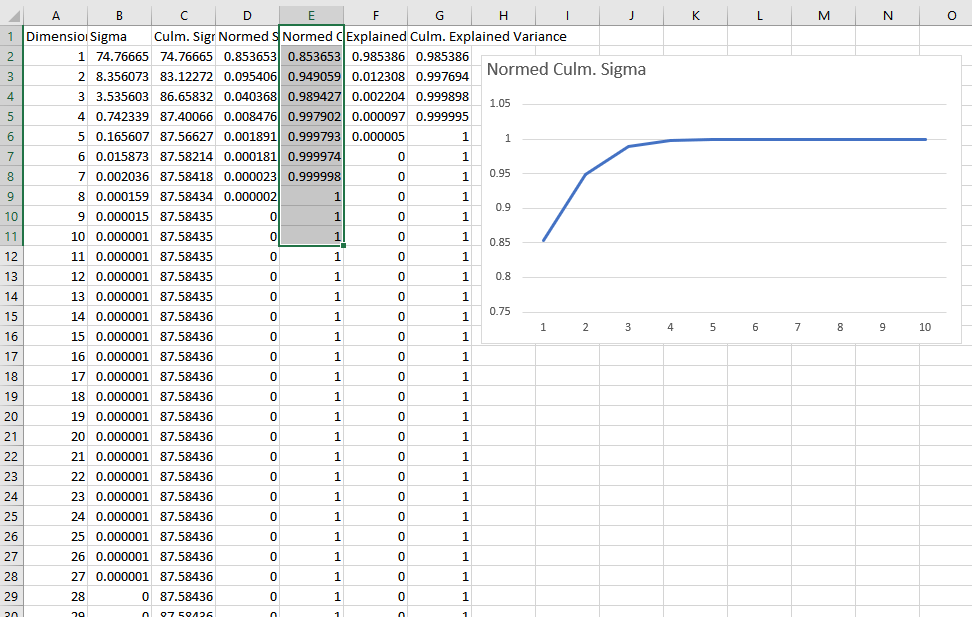
The last 2 columns in this data show “Explained Variance” and “Culmulative Explained Variance” which is another metric to use to see how good a fit is for a certain number of dimensions. You calculate explained variance by dividing sigma squared by the sum of all sigmas squared. For culmulative explained variance, you sum up the sigmas squared at or before the dimension you are looking at, divided by the sum of all sigmas squared.

An intuitive perspective to SVD for data compression is that if you have some data that is AxB in size, SVD will break it into three matrices: an AxA matrix, an AxA scaling matrix, and an AxB matrix. You can multiply the middle scaling matrix into either the left or the right matrix and then end up with only two matrices: one is AxA and the other is AxB. At this point, our data is larger than it used to be, but that scaling matrix told us how important each column of the first matrix / row of the second matrix is. We can remove those for any place that the scaling matrix is zero or close enough to zero to be considered zero. That gives us two matrices AxN and NxB. At this point, if (A*N + N*B) is smaller than (A*B) then we’ve compressed our data in a nearly lossless way.

We don’t have to stop here though, and can start trimming more rows and columns off to make the matrices be AxM and MxB, such that (A*M + M*B) is smaller than (A*B) by as much as we want – but we introduce error into the process and our compression is no longer lossless. The error we are adding is minimized in the “least squares” sense, so it will be many small errors instead of a few large errors, which is often desired in practice.

A matrix multiply is all that is needed to get your data back, but individual values can be read back easily as well (random access). You get the a’th row from the first matrix, and the b’th column from the second matrix. The vectors will both be of size M. You dot product them, and your value is “decompressed”.

If doing something like compressing animation, the first matrix might be indexed by time, and the second matrix might be indexed by bone id*3, having 3 entries for the position of a bone starting at that bone id*3 location in the matrix. Then it’s just a vec3 * mat3x3 multiply (or alternately 3 dot products) to get the position back.

Shorter Intuition & Practical Concerns (Added 10/2/22)

Here is some shorter intuition for using truncated SVD for data compression.

If you start with data that is W * H in size, this lets you make it into data that is (W + H) * N in size, where N is tuneable for quality vs size. The U matrix will be W * N in size, and the SigmaV matrix will be H * N in size.

To decompress a single value at (X,Y), you read an N sized vector from U, an N sized vector from SigmaV, and dot product them to get the value back.

The downside to this technique is the memory (texture) reads, where for each value you want to decompress you need to read 2*N values to dot product them together.

Closing And Links

The Eigen library is pretty neat. You can grab the latest zip from https://eigen.tuxfamily.org/ and after unzipping, the “Eigen” folder within the zip has the files you want to include in your program.

Compilation times are pretty long when including files from this library, which i found surprising. It’d probably be best to put the includes to Eigen within a static library that didn’t get changed often to avoid the compilation times. I also had to turn on \bigobj in msvc after hitting an error regarding it.

Other than that, I’m a fan of Eigen and expect to use it when I need to do things like this, instead of writing from scratch, or calling into python scripts to do these numerical operations (hehe).

Here is a great use of SVD to compress PBR textures:
https://bartwronski.com/2020/05/21/dimensionality-reduction-for-image-and-texture-set-compression/

Here are some links I found useful when learning SVD:
https://jonathan-hui.medium.com/machine-learning-singular-value-decomposition-svd-principal-component-analysis-pca-1d45e885e491 
https://youtu.be/DG7YTlGnCEo
https://youtu.be/Jqg7JgCwQrk
https://towardsdatascience.com/simple-svd-algorithms-13291ad2eef2 
https://medium.com/swlh/truncated-singular-value-decomposition-svd-using-amazon-food-reviews-891d97af5d8d