The source code that goes with this post can be found at https://github.com/Atrix256/EulerProbability

A few weeks ago I saw a great video on youtube that showed how Euler’s number e comes up everywhere.
https://www.youtube.com/watch?v=AAir4vcxRPU

It was a lot of the same old stuff we’ve all seen many times before but then started talking about Euler’s number showing up in probability. The video instantly had my full attention.

I spend a lot of time thinking about how uses of white noise can be turned into using blue noise or low discrepancy sequences because white noise has nice properties at the limit, but those other things have the same properties over much smaller numbers of samples. This link to probability made we wonder how other types of noise / sequences would behave when put through the same situations where Euler’s number emerged. Would e still emerge, or would it be a different value for different sequence types?

This is what sent me on the rabbit hole for the two prior blog posts, which explore making streaming uniform red noise, blue noise, and other random number generators.

Let’s get into it!

Lottery Winnings

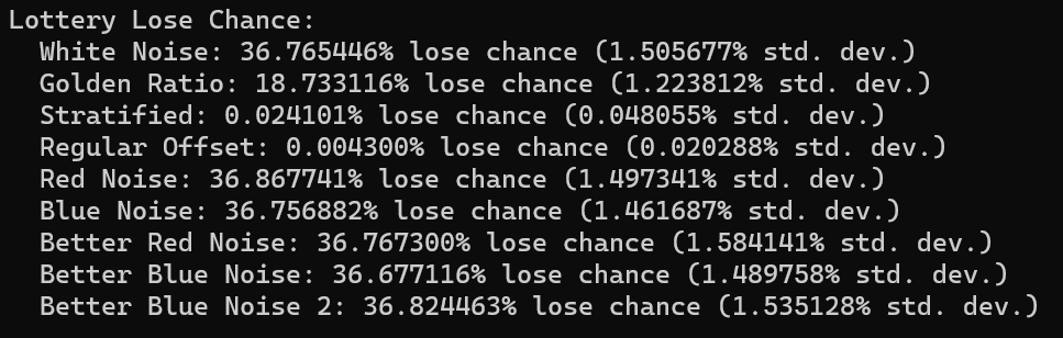
One claim the video makes is that if the odds for winning the lottery are 1 in N, that if you buy N lottery tickets, there is a 1/e chance that you will still lose. 1/e is 0.367879, so that is a 36.79% of losing.

That may be true for white noise, but how about other sequences?

To test, I generate a random integer in [0,N) as the winning number, and then generate N more random numbers as the lottery tickets, each also in [0, N). The test results in a win (1) or a loss (0). This test is done 1,000,000 times to get an average chance of losing. Also, standard deviation is calculated by looking at the percentage of each group of 1,000 tests.

Here are the sequences tested:

• White Noise – regular old random numbers
• Golden Ratio – the deterministic golden ratio sequence: fract(index * phi)
• Stratified – stratify N buckets to make N numbers
• Regular Offset – N regularly spaced numbers, but with a random offset and modulus to keep them in range.
• Red Noise – made by adding two values together, converting from triangle to uniform, and rerolling one of the numbers for next time. Each number gets regenerated every other index. (https://blog.demofox.org/2023/02/20/uniform-1d-red-noise-blue-noise/)
• Blue Noise – made by subtracting one value from another, converting from triangle to uniform, and rerolling one of the numbers for next time. Each number gets regenerated every other index, and which value gets subtracted changes each index as well. (https://blog.demofox.org/2023/02/20/uniform-1d-red-noise-blue-noise/)
• Better Red Noise – FIR filtered white noise, with a piecewise polynomial to transform it back to uniform. (https://blog.demofox.org/2023/03/06/uniform-1d-red-noise-blue-noise-part-2/)
• Better Blue Noise – FIR filtered white noise, with a piecewise polynomial to transform it back to uniform. (https://blog.demofox.org/2023/03/06/uniform-1d-red-noise-blue-noise-part-2/)
• Better Blue Noise 2 – IIR filtering white noise, from Nick Appleton (https://blog.demofox.org/2023/03/06/uniform-1d-red-noise-blue-noise-part-2/)

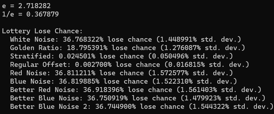
We were able to duplicate the results for white noise which is neat. Using the golden ratio sequence cuts the loss rate in half. I chalk this up to it being more fairly distributed than white noise. White noise is going to give you the same lottery ticket number several times, where golden ratio is going to reduce that redundancy.

Stratified and regular offset both did very well on this test, but that isn’t surprising. If you have a 1 in N chance of picking a winning random number, and you make (almost) every number between 1 and N as a guess, you are going to (almost) always win. The little bit of randomization in each will keep them from winning 100% of the time.

the red noise and blue noise were very close to having a 1/e loss chance but were off in the tenths of a percentage place. Running it again gives similar results, so I think this could be a real, but small, effect. Colored noise seems like it affects this outcome a little bit.

Summing Random Values

Another claim the video makes is that if you add random uniform white noise numbers together, it will on average take e of them (2.718282) to be greater than or equal to 1. I do that test 100,000,000 times with each sequence again.

Let’s see:

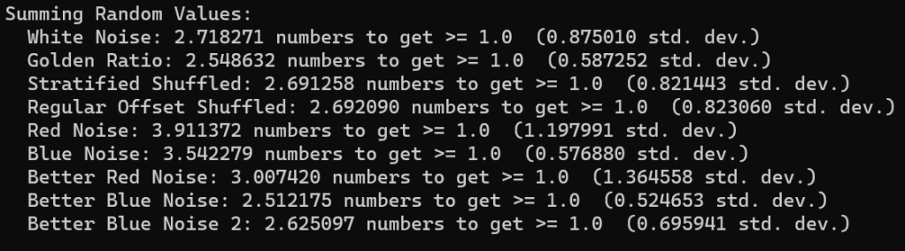
We duplicated the results with white noise again, which is neat.

The golden ratio sequence takes slightly fewer numbers to reach 1.0. Subsequent numbers of the golden ratio sequence are pretty different usually, so this makes some sense to me.

For stratified and regular offset, I wanted to include them, but their sequence is in order, which doesn’t make sense for this test. So, I shuffled them. The result looks to be just a little bit lower than e.

The lower quality red and blue noise took quite a bit more numbers to reach 1.0 at 3.9 and 3.5 respectively. The better red noise took 3 numbers on average, while the blue noise took the lowest seen at 2.5 numbers. Lastly, the FIR blue noise “better blue noise 2” took just under e.

An interesting observation is that the red noises all have higher standard deviation than the other sequences. Red noise makes similar numbers consecutively, so if the numbers are smaller, it would take more of them, where if they were bigger it would take fewer of them. I think that is why the standard deviation (square root of variance) is higher. It’s just more erratic.

Contrary to that, the blue noise sequences have lower standard deviation. Blue noise makes dis-similar numbers consecutively, so I think it makes sense that it would be more consistent in how many numbers it took to sum to 1.0, and thus have a lower standard deviation and variance.

Finding The Best Scoring Item

The video also had this neat algorithm for fairly reliably finding the best scoring item, without having to look at all items.

Their setup is that you have job applicants to review and after talking to each, you have to decide right then to hire the person or to continue looking at other candidates. The algorithm is that you interview 1/e percent of them (36.79%), not hiring any of them, but keeping track of how well the best interviewer did. You then start interviewing the remaining candidates and hire the first one that does better than the previous best.

Doing this apparently gives you a 1/e (36.79%) chance of picking the actual best candidate, even though you don’t evaluate all the candidates. That is pretty neat.

I did this test 10,000,000 times for each sequence type

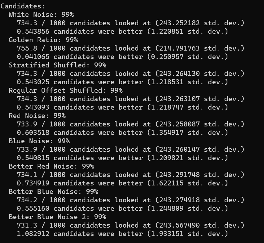
All sequence types looked at 733 or 734 candidates out of 1000 on average. The golden ratio sequence actually ended up looking at 755 on average though, and the better blue noise 2 sequence looked at 731. The standard deviation is ~243 for all of them, except for golden ratio which is 214. So… golden ratio looks at more candidates on average, but it’s also more consistent about the number of candidates it looks at.

Most sequence types had roughly 0.5 candidates on average better than the candidate hired. The golden ratio has 0.04 candidates better on average though. Red noise has slightly more candidates better than that though, at 0.6 and 0.73. The “Better Blue Noise 2” has a full 1.08 candidates better on average. The standard deviation follows these counts… golden ratio is the lowest standard deviation by far, red noise is higher than average, and the better blue noise 2 is much higher than the rest.

Closing

As usual, the lesson is that DSP, stochastic algorithms and sampling are deep topics.

Did I miss something, or is there something I should know? Leave a comment here or hit me up on mastodon at https://mastodon.gamedev.place/@demofox