The code that made the diagrams in this post can be found at https://github.com/Atrix256/ToroidalProgressiveStratification1D

I stumbled on this when working on something else. I’m not sure of a use case for it, but I want to share it in case there is one I’m not thinking of, or in case it inspires other ideas.

Let’s say you want to do Monte Carlo integration on a function y=f(x) for x being between 0 and 10. You can do this by choosing random values for x between 0 and 10, and averaging the y values to get an “average height” of the function between those two points. This leaves you with a rectangle where you know the width (10) and you are estimating the height (the average y value). You just multiply the width by that estimated height to get an estimate of the integral. The more points you use, the more accurate your estimate is. You can use Monte Carlo integration to solve integrals that you can’t solve analytically.

For deeper information Monte Carlo integration including importance sampling, give this a read: https://blog.demofox.org/2018/06/12/monte-carlo-integration-explanation-in-1d/

We use Monte Carlo integration A LOT in rendering, and specifically real time rendering. This is especially true in the modern age of ray traced rendering. When a render is noisy, what you are seeing is the error from Monte Carlo integration not being accurate enough with the number of samples we can afford computationally. We then try to fix the noise using various methods, such as filtering and denoising, or by changing how we pick the x values to plug in (better sampling patterns). Here are some relevant resources:

• When Random Numbers Are Too Random: Low Discrepancy Sequences – https://blog.demofox.org/2017/05/29/when-random-numbers-are-too-random-low-discrepancy-sequences/
• “Beyond White Noise for Real-Time Rendering” (YouTube) – https://www.youtube.com/watch?v=tethAU66xaA
• “Importance-Sampled Filter-Adapted Spatio-Temporal Sampling” – https://github.com/electronicarts/importance-sampled-FAST-noise

Let’s say we want to integrate the function y=f(x) where x is a scalar value between 0 and 1. Three common ways to do this are:

1. Uniform White Noise – Use a standard random number generator (or hash function) to generate numbers between 0 and 1.
2. Golden Ratio – Starting with any value, add the golden ratio to it (1.6180339887…) and throw away the whole numbers (aka take the result mod 1) to get a random value (quasirandom technically). repeat to get more values.
3. Stratified – If you know you want to take N samples, break the 0 to 1 range into N equally sized bins, and put one uniform white noise value in each bucket. Like if you wanted to take two samples, you’d have a random number between 0 and 1/2, and another between 1/2 and 1. A problem with uniform white noise is that it tends to clump up and leave big holes. Stratification helps make the points more evenly spaced.

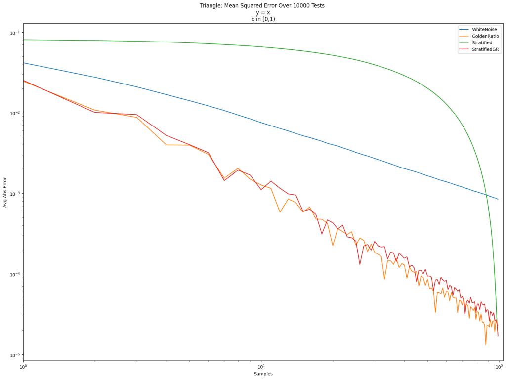
Here’s a log/log error graph using those 3 kinds of sampling strategies to integrate the function y=x from 0 to 1. The x axis is the number of samples, and the y axis is error.

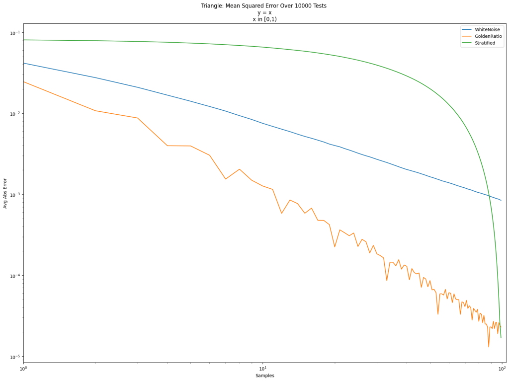
White noise is terrible as usual. Friends don’t let friends use white noise. The golden ratio sequence is great, as per usual. Golden ratio for the win! Stratification is also quite good, but it doesn’t give very good results until the end.

Stratified sampling doesn’t do well in the middle because we are picking points in order. Like for 100 points, we sample between 0 and 1/100, then between 1/100 and 2/100, then between 2/100 and 3/100 and so on. By the end it fills in the space between 0 and 1, but it takes a while to get there.

The question is… can we make stratified sampling that is good all along the way, instead of only being good at the end? The answer is yes we can.

An observation is that we could visit those bins in a different order. But what order should we visit them in? We are going to get a bit meta and visit them in “golden ratio” order. If are taking N samples, we are going to pretend that N is 1.0, and we are going to do golden ratio sampling to pick the order of the buckets to do stratified sampling in. If we naively used the golden ratio sequence, multiplied by N and cast to integer to get the bucket index, we’d find we hit some of the buckets multiple times, and missed some of the buckets. But it turns out that we can find an integer coprime to N that is closest to the golden ratio. We can then start at any index, and repeatedly add that number to our index to get the next index – making sure to take the result modulo N. We will then visit each bucket exactly once before repeating the sequence.

That’s a brief description of a low discrepancy shuffle iterator I wrote up on a previous blog post: https://blog.demofox.org/2024/05/19/a-low-discrepancy-shuffle-iterator-random-access-inversion/.

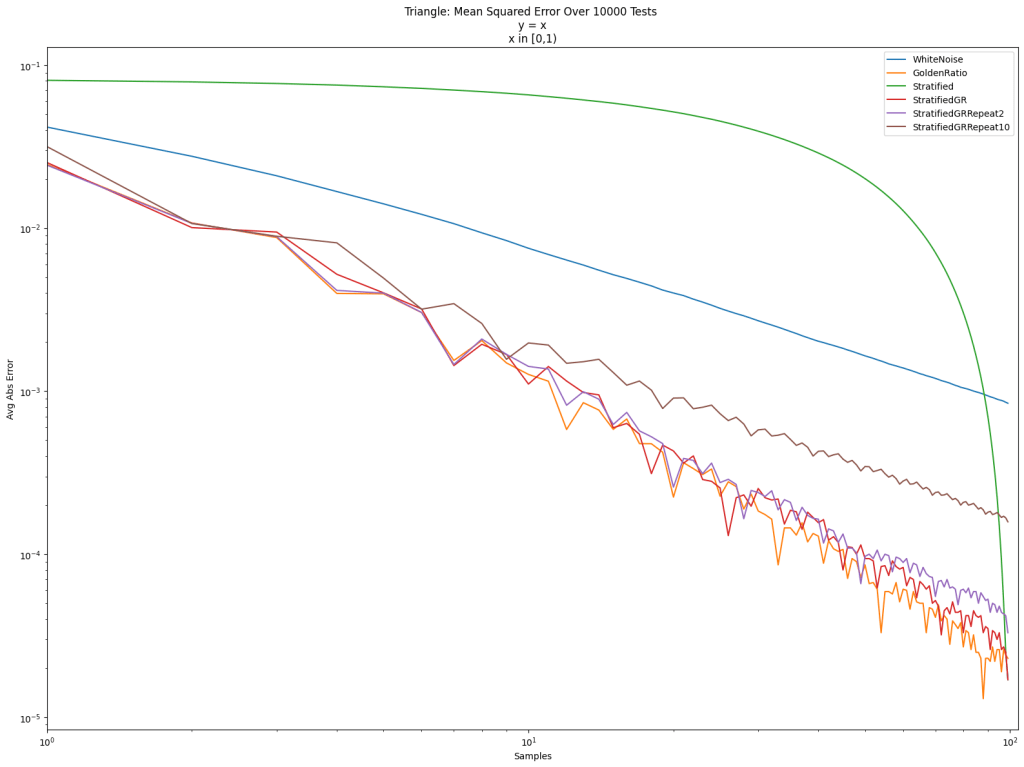
Doing that, we get “StratifiedGR” below. It does nearly as well as the golden ratio sequence, but the final result is the same as if we did stratification in order.

Is this useful? Well, it’s hard to tell in general whether stratified sampling or golden ratio wins for taking N samples in Monte Carlo integration.

The golden ratio (orange) is usually lower error than the golden ratio shuffled stratifed sampling (red), but the ending error is 0.000017 for “StratifedGR” (same as Stratified), while it is 0.000023 for “GoldenRatio” (and 0.000843 for “WhiteNoise”), so stratification has lower error in the end.

A nice thing about the golden ratio sequence is that you can always add more points to the sequence, where for stratified sampling – and even golden ratio shuffled stratified sampling – you have to know the number of samples you want to take in advance and can’t naturally extend it and add more.

Stratifed sampling is randomized within the buckets, so we could repeat the sequence again to get new samples, but we are using the same buckets, and we are putting white noise values in them, so our sequence just sort of gets “white noise gains”, instead of the gains that a progressive, open, low discrepancy sequence gives. Below we repeat golden ratio shuffled stratification twice (purple) and 10 times (brown). You can see that golden ratio shuffled stratification loses quality when you repeat it. You really need to know how many samples you want at max, when doing golden ratio shuffled stratified sampling, but you are free to use less than than number.

By doing a golden ratio shuffle on stratified sampling, we did make it progressive (“good” at any number of samples), but we also made it progressive from any index (“good” starting from any index, for any number of samples). That is a pretty neat property, and comes from the fact that our golden ratio shuffle iterator is actually a rank 1 lattice, just like the actual golden ratio sequence, and this is a property of all rank 1 lattices.

However, by golden ratio shuffling stratification, we also made it TOROIDALLY progressive. What i mean by that is that the sampling sequence is finite, but that you can start at any index and have “good” sampling for any number of samples EVEN WHEN THE SEQUENCE FINISHES AND STARTS OVER. There is no “seam” when this sequence starts over. It just keeps going at the full level of quality. This is due to the fact that our “golden ratio shuffle iterator” rank 1 lattice uses a number that is coprime to N to visit all the indicies [0, N) exactly once before repeating.

This torodial progressiveness is useful if you have a lot of things doing integration at once, all using the same sampling sequence for the function, but individually, they may be (re)starting integration on different time intervals. That may sound strange and exotic, but that is exactly what is happening in temporal anti aliasing (TAA). We have a global sub pixel camera jitter, which is the x we plug into the y=f(x) as we integrate every pixel over its footprint, but each pixel individually uses neighborhood color clamping and other heuristics to decide when it should throw out the integration history and start over.

The only challenge is that if we wanted to use something like this for TAA, we would need a 2D sequence for the camera jitter instead of 1D. I do happen to have a blog post on a 2D version of the low discrepancy shuffler. I don’t think that will magically be the answer needed here, but perhaps you can smell what I’m cooking 😛

A Two Dimensional Low Discrepancy Shuffle Iterator (+Random Access & Inversion): https://blog.demofox.org/2024/10/04/a-two-dimensional-low-discrepancy-shuffle-iterator-random-access-inversion/

I should note there are other ways to do progressive stratified sampling, for instance the great 2018 paper “Progressive Multi-Jittered Sample Sequences” by Per Christensen, Andrew Kensler and Charlie Kilpatrick. https://graphics.pixar.com/library/ProgressiveMultiJitteredSampling/paper.pdf

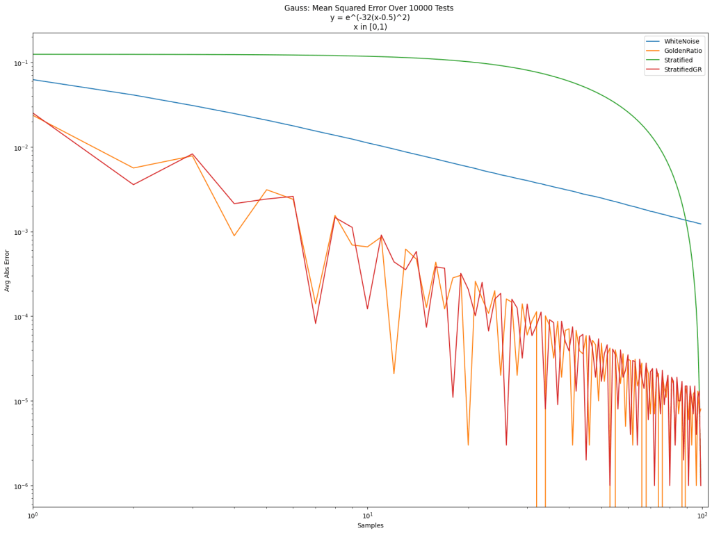
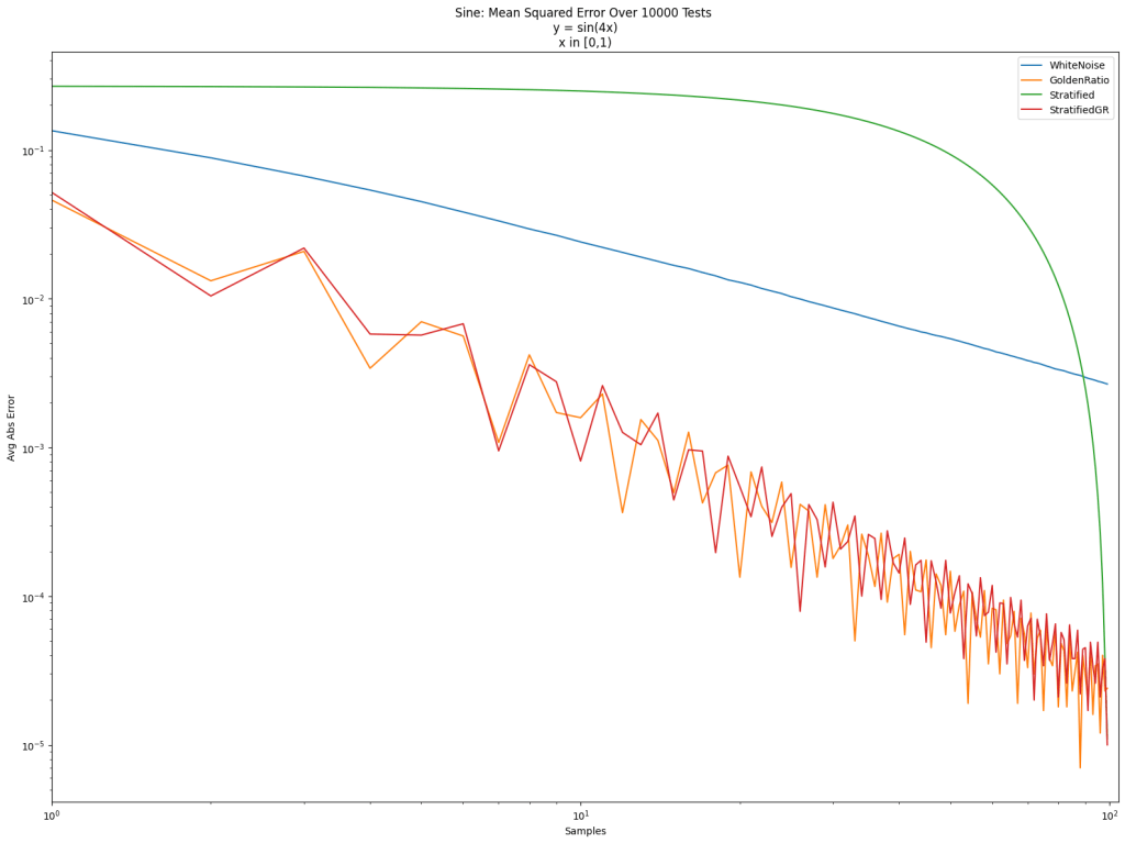
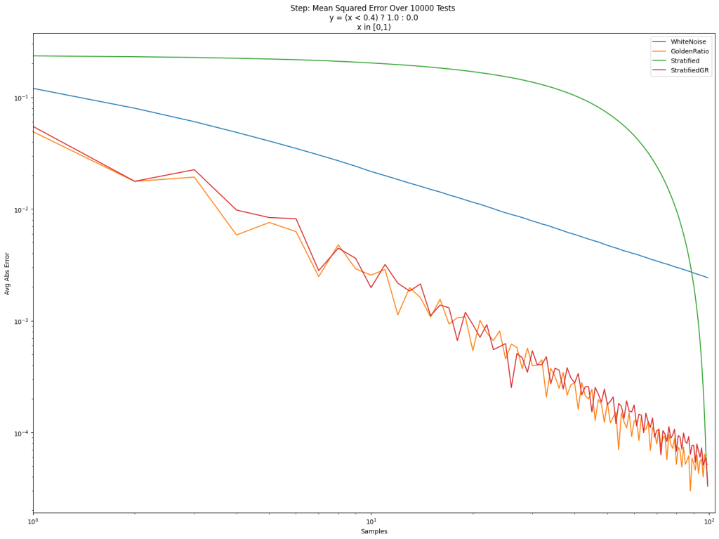
In the post so far, we’ve only looked at integrating the “triangle” function y=x. Below are the results for that again, and also for a step function, a sine function, and a Gaussian function. Different sampling sequences behave better or worse with different types of integrands sometimes.

Final Error Amounts:

	Gauss	Sine	Step	Triangle
WhiteNoise	0.001232	0.002671	0.002425	0.000843
GoldenRatio	0.000008	0.000024	0.000052	0.000023
Stratified	0.000001	0.000011	0.000033	0.000017
StratifiedGR	0.000001	0.000011	0.000033	0.000017