Rectangular Bezier Patches

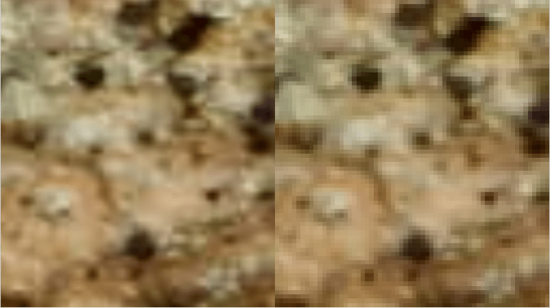
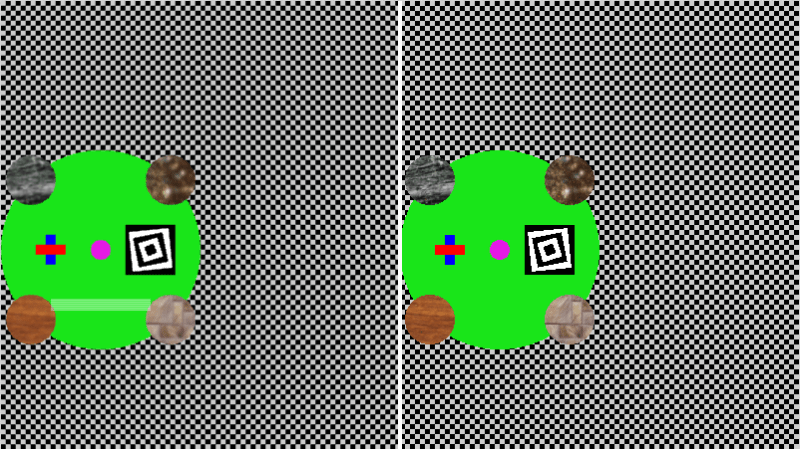
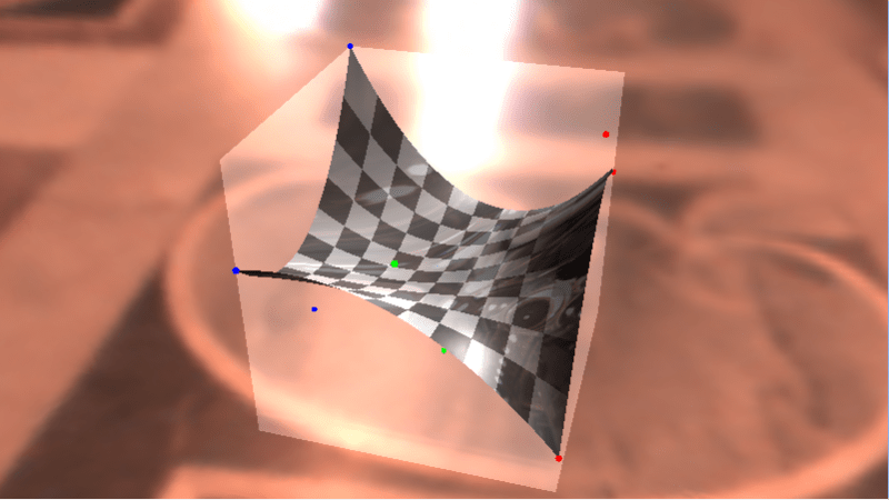
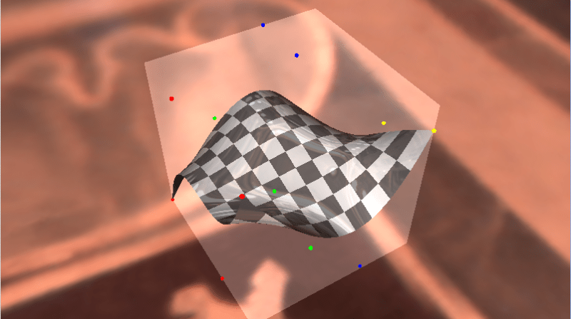
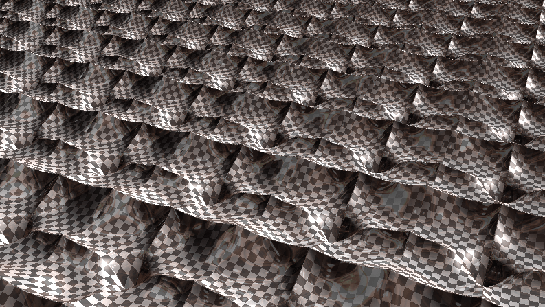
Rectangular Bezier Patches are one way to bring Bezier curves into the 3rd dimension as a Bezier surface. Below is a rendered image of a quadratic Bezier rectangle (degree of (2,2)) and a cubic Bezier rectangle (degree of (3,3)) taken as screenshots from a shadertoy demo I created that renders these in real time. Links at bottom of post!


Intuition

Imagine that you had a Bezier curve with some number of control points. Now, imagine that you wanted to animate those control points over time instead of having a static curve.

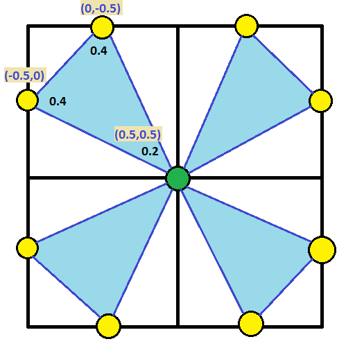
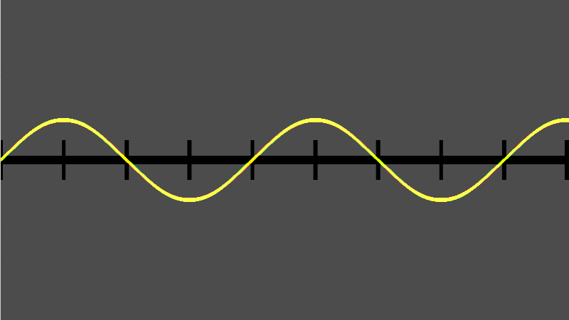
One way to do this would be to just have multiple sets of control points as key frames, and just linearly interpolate between the key frames over time. You’d get something that might look like the image below (lighter red = farther back in time).

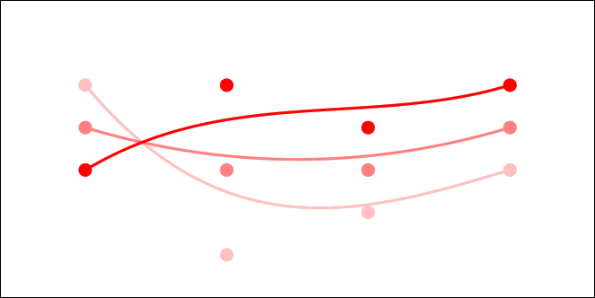
That is a simple and intuitive way to animate a Bezier curve, and is probably what you thought of immediately. Interestingly though, since linear interpolation is really a degree 1 Bezier curve, this method is actually using a degree 1 Bezier curve to control each control point!

What if we tried a higher order curve to animate each control point? Well… we could have three sets of control points, so that each control point was controlled over time by a quadratic curve. We could also try having four sets of control points, so that each control point was controlled over time by a cubic curve.

We could have any number of sets of control points, to be able to animate the control points over time using any degree curve.

Now, instead of animating the curve over TIME, what if we controlled it over DISTANCE (like, say, the z-axis, or “depth”). Look at the image above and think of it like you are looking at a surface from the side. If you took a bunch of the time interpolations as slices and set them next to each other so that there were no gaps between them, you’d end up with a smooth surface. TA-DA! This is how a Rectangular Bezier Patch is made.

Note that the degree of the curve on one axis doesn’t have to match the degree of the curve on the other axis. You could have a cubic curve where each control point is controlled by a linear interpolation, or you could have a degree 5 curve where each control point is controlled by degree 7 curves. Since there are two degrees involved in a Bezier rectangle, you describe it’s order with two numbers. The first example is degree (3,1) and the second example is degree (5,7).

Higher Dimensions

While you thinking about this, I wanted to mention that you could animate a bezier rectangle over time, using bezier curves to control those control points. If you then laid that out over distance instead of time, you’d end up with a rectangular box Bezier solid. If you are having trouble visualizing that, don’t feel dumb, it’s actually four dimensional!

You can think of it like a box that has a value stored at every (x,y,z) location, and those values are controlled by Bezier formulas so are smooth and are based on control points. It’s kind of a strange concept but is useful in some situations.

Say you made a 3d hot air baloon game and wanted to model temperature of the air at differently locations to simulate thermals. One way you could do this would be to store a bunch of temperatures in a 3d grid. Another way might involve using a grid of rectangular box Bezier solids perhaps. One benefit to the Bezier solid representation is that the data points are much smoother than a grid would be, and another is that you could make the grid much less dense.

Now, let’s say that you wanted to animate the thermals over time. You could use a fifth dimensional bezier hypercube solid. Let’s move on, my brain hurts 😛

Math

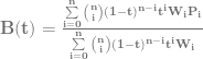
The equation for a Bezier Rectangle is:

\mathbf{p}(u, v) = \sum_{i=0}^n \sum_{j=0}^m B_i^n(u) \; B_j^m(v) \; \mathbf{k}_{i,j}

\mathbf{p}(u, v) is the point on the surface that you get after you plug in the parameters. u and v are the parameters to the surface and should be within the range 0 to 1. These are the same thing as the t you see in Bezier curves, but there are two of them since there are two axes.

There are two Sigmas (summations) which mean that it’s a double for loop.

One of the for loops make i go from 0 to n and the other makes j go from 0 to m. m and n are the degree of each axis.

B_i^n(u) and B_i^n(u) are Bernstein polynomials (aka binomial expansion terms) just as you see in Bezier Curves – there is just one per axis.

Lastly comes the control points \mathbf{k}_{i,j}. The number of control on one axis are multiplied by the number of control points on the other axis.

A biquadratic Bezier patch has a degree of (2,2) and has 3 control points on one axis, and 3 control points on the other. That means that it has 9 control points total.

A bicubic Bezier patch has a degree of (3,3) with 4 control points on each axis, for a total of 16 control points.

If you had a patch of degree (7,1), it would have 8 control points on one axis and 2 control points on the other axis, and so would also have 16 control points total, but they would be laid out differently than a bicubic Bezier patch.

As far as actually calculating points on a curve, the above only calculates the value for a single axis for the final point on the curve. If you have three dimensional control points (X,Y,Z), you have to do the above math for each one to get the final result. This is the same as how it works for evaluating Bezier curves.

Code

#include 
#include 

typedef std::array TFloat3;
typedef std::array TFloat3x3;

const TFloat3x3 c_ControlPointsX =
{
    {
        { 0.7f, 0.8f, 0.9f },
        { 0.2f, 0.5f, 0.4f },
        { 0.6f, 0.3f, 0.1f },
    }
};

const TFloat3x3 c_ControlPointsY =
{
    {
        { 0.2f, 0.8f, 0.5f },
        { 0.6f, 0.9f, 0.3f },
        { 0.7f, 0.1f, 0.4f },
    }
};

const TFloat3x3 c_ControlPointsZ =
{
    {
        { 0.6f, 0.5f, 0.3f },
        { 0.7f, 0.1f, 0.9f },
        { 0.8f, 0.4f, 0.2f },
    }
};

void WaitForEnter ()
{
    printf("Press Enter to quit");
    fflush(stdin);
    getchar();
}

float QuadraticBezier (const TFloat3& p, float t)
{
    float s = 1.0f - t;
    float s2 = s * s;
    float t2 = t * t;

    return
        p[0] * s2 +
        p[1] * 2.0f * s * t +
        p[2] * t2;
}

float BiquadraticBezierPatch(const TFloat3x3& p, float u, float v)
{
    TFloat3 uValues;
    uValues[0] = QuadraticBezier(p[0], u);
    uValues[1] = QuadraticBezier(p[1], u);
    uValues[2] = QuadraticBezier(p[2], u);
    return QuadraticBezier(uValues, v);
}

int main(int argc, char **argv)
{
    // how many values to display on each axis. Limited by console resolution!
    const int c_numValues = 4;

    printf("Bezier rectangle:n");
    for (int i = 0; i < c_numValues; ++i)
    {
        float iPercent = ((float)i) / ((float)(c_numValues - 1));
        for (int j = 0; j < c_numValues; ++j)
        {
            if (j == 0)
                printf("  ");
            float jPercent = ((float)j) / ((float)(c_numValues - 1));
            float valueX = BiquadraticBezierPatch(c_ControlPointsX, jPercent, iPercent);
            float valueY = BiquadraticBezierPatch(c_ControlPointsY, jPercent, iPercent);
            float valueZ = BiquadraticBezierPatch(c_ControlPointsZ, jPercent, iPercent);
            printf("(%0.2f, %0.2f, %0.2f) ", valueX, valueY, valueZ);
        }
        printf("n");
    }
    printf("n");

    WaitForEnter();
    return 0;
}

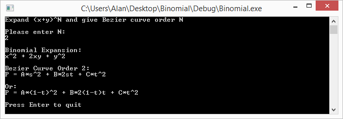
And here is the output it gives:

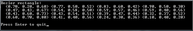
Note that in the program above, I evaluate the surface points by evaluating one axis and then the other. This is basically the same as how I explained it at the top, where I’m effectively animating the control points over distance, then evaluating the curve slice of the surface at that specific distance.

You could also write it another way though, where you literally expand the mathematical formula to get just one expression to evaluate that takes all control points at once. I like the simplicity (of understanding) of the method I used, but the other method works just as well.

The Rendering

It’s easy enough to calculate values on a Bezier Rectangle, but what if you want to draw one?

One way is to tessellate it, or break it up into triangles and then render the triangles. You can think of it like trying to render a grid, where each point of the grid is moved to be where ever the Bezier rectangle function says it should be.

Raytracing against these objects in the general case is very difficult however, because it basically comes down to solving equations of very high degree.

Raymarching against these objects is also difficult unfortunately because while raymarching only needs to know “am i above the shape, or underneath it?”, knowing what u,v to plug into the equation to get the height most relevant to a random point in space is also very difficult. Not as difficult as the raytracing equations, but probably just as much out of reach.

But never fear, as always, you can cheat!

If you read my post about one dimensional (explicit) Bezier curves (One Dimensional Bezier Curves), you may remember that math gets easier if you use one dimensional control points. The same is actually true with Bezier rectangles!

For the ray marching case, you can march a point through space, and plug the x,z coordinate of the point into the Bezier rectangle function as u,v values and the number that comes out you can treat as a y coordinate.

Now, ray marching a Bezier rectangle is the same as ray marching any old height map (check links section for more info on that).

What I did in my demos, is since i knew that the curve was constrained to 0-1 on the x and z axis, and the y axis min and max was the control point min and maxes, I did a raytrace of that bounding box to get a minimum and maximum distance that the ray was inside that box. From there, I did raymarching from that min time to the max time along the ray, considering the ray as hitting the surface whenever the distance from the ray to the surface on the y axis (rayPos.y – bezierRectangle.y) changed sign.

After I had a hit, I got the height of the curve slightly offset on the x axis, then slightly offset on the z axis to get a triangle that I could calculate a surface normal from, to do lighting and shading with.

There is room for improvement in the ray marching though. I evenly divide the space through the box by a specific amount to control the size of the steps. A better way to do this I think would be to get the gradient of the function and use that to get a distance estimate (check links section below for more information). I could use that value to control the distance the ray marches at each step, and should be able to march through the box much quicker.

Also, as the link on terrain marching explains, you can usually take farther steps when the ray is farther from the camera, because the eye notices less detail. I removed that since the Bezier rectangles are pretty close to the camera, but it probably still would be helpful. Also, it would DEFINITELY be helpful in the case of the “Infinite Bezier Rectangles” scene.

I am pretty sure you could directly raytrace an explicit Bezier rectangle (one who has one dimensional control points) – at least for low degrees. I personally don’t know how you would do that, but I think it might boil down to solving a 4th degree function or something else “reasonable” based on a similar question I had about Bezier triangles on the mathematics stack exchange site (link below).

Another Way To Render

There is another way to render Bezier surfaces using ray based methods that I didn’t use but want to mention.

A property of Bezier curves and surfaces is that they are guaranteed to be completely contained by the convex hull created by their control points.

Another property of Bezier curves and surfaces is that you can use the De Casteljeau algorithm to cut them up. For instance you could cut a Bezier curve into two different Bezier curves, and the same holds for Bezier surfaces.

Using these two properties, there is an interesting way to be able to tell if a ray intersects a bezier curve or not, which is:

  1. If the line misses the convex hull, return a miss
  2. If the convex hull is smaller than a pixel, return a hit
  3. Otherwise, cut the Bezier object into a couple smaller Bezier objects
  4. Recurse for each smaller Bezier object

Yes, believe it or not, that is a real technique! It’s called Bezier Clipping and there is a research paper in the links section below that talks about some of the details of using that rendering technique.

Links

Lastly, I wanted to mention that the above is completely about Bezier rectangles, but there is no reason you couldn’t extend these rectangles to use rational Bezier functions, or be based on B-splines or NURBS, or even go a different direction and make hermite surfaces or catmull-rom surfaces, or even make surfaces that used exotic basis functions of your own crafting based on trigonometric functions or whatever else!

Here are the shadertoy demos I made:
Shadertoy: Cubic Bezier Rectangle
Shadertoy: Quadratic Bezier Rectangle
Shadertoy: Infinite Bezier Rectangles

And some other links about this stuff:
IQ – terrain raymarching
IQ – distance estimation (using function gradients)
Math Stack Exchange – Ray intersection with explicit (1 axis) Bezier triangle?
Math Stack Exchange – Intersect Ray (Line) vs Quadratic Bezier Triangle
Bézier Surfaces: de Casteljau’s Algorithm
Ray Tracing Triangular Bézier Patches (including Bezier clipping)
Wikipedia: Bezier Surface
Wikipedia: Bezier Triangle

Lagrange Interpolation

Lagrange interpolation is a way of crafting a function from a set of data points..

In the past I’ve seen reference to Lagrange interpolation in relation to audio programming like, for helping make a soft knee for a limiter, but it can be used wherever you need to make a function from some data points.

What’s It Do?

Lagrange interpolation is a way of crafting a y=f(x) function from a set of (x,y) data pairs. The resulting function passes through all the data points you give it (like a Catmull-Rom spline does), so can be used to find a function to interpolate between data sets.

You can’t give two value pairs that have the same x value, but the data points don’t have to be evenly spaced.

Also, if you give N data points, you’ll get out a function that is a N-1 degree polynomial. So, if you interpolate two data points, you’ll get a degree 1 polynomial (a line). If you interpolate three data points, you’ll get a degree 2 polynomial (a quadratic).

The function will be quite messy, but you can use algebra, or wolframalpha.com (or the like) to simplify it for you to a simpler equation.

Lagrange interpolation is subject to Runge’s Phenomenon, so the more data points you have, the more the interpolation tends to get “squirly” near the edges and shoot off up high or down low, instead of smoothly interpolating between data values.

How’s It Do It?

Well, to make any kind of curve from data points, if we want the curve to pass through those data points, one way would be to come up with a set of functions to multiply each data point by.

Each function must evaluate to 1 when the curve is at that control point, it should be zero when the curve is at any other control point. Between control points, the function can take any value, but if you make it continuous / smooth, the curve will be continuous and smooth, so that’s usually what is desired.

When we have those functions, to get a point on the curve we just multiply each control point by it’s corresponding function (called a basis function), and we sum up the results.

The pseudocode below is how this works and is the basic functionality of most common curve types:

// The basic way to evaluate most any type of curve
float PointOnCurve (float t, float *controlPoints, int numControlPoints)
{
    float value = 0.0f;

    for (int i = 0; i < numControlPoints; ++i)
        value += controlPoints[i] * ControlPointFunction(i, t);

    return value;
}

float ControlPointFunction (int i, float t)
{
  // return the ith control point function evaluated at time t.
  // aka return f(t) for the ith control point.
}

What makes Lagrange interpolation different than other curve types is the basis functions it uses.

The Math

If you aren’t used to seeing a capital pi, or a laplacian style cursive l in equations, it’s about to get a bit mathy!

If you feel like skipping to the next section, I don’t blame you, but if you are feeling brave, you should try and follow along, because I’m going to slowly walk through each and every symbol to help explain what’s going on and why.

Let’s say that you are want to be able to interpolate between k+1 data points:

(x_0, y_0)\ldots(x_k, y_k)

The formula for calculating a Lagrange interpolated value is this:

L(x) := \sum_{j=0}^{k} y_j \ell_j(x)

The capital sigma (\sum_{j=0}^{k}
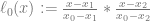
) just means that we are going to loop a variable j from 0 to k (including k), and we are going to sum up the total of everything on the right for all values of j. When you see a capital sigma, think sum (note they both start with an s).

The next thing after the sigma is y_j. That is just the y value from our jth control point. That is essentially controlPoints[j].y.

After that comes the last part \ell_j(x)
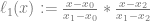
. That is just the function for the jth control point that we multiply the control point by (aka the basis function), evaluated for the specific value x.

Since there is no operator between this function and the control point, that means we multiply them together. So yeah… that crazy math just says “multiply each control point by it’s basis function, and sum up the results”, just like our pseudo code above does!

The second equation we need to look at is the definition of the basis functions for each control point. Here is the formula that describes the jth basis function, for the jth control point:

\ell_j(x) := \prod_{\begin{smallmatrix}0\le m\le k\\ m\neq j\end{smallmatrix}} \frac{x-x_m}{x_j-x_m}

First is the capital pi \prod_{\begin{smallmatrix}0\le m\le k\\ m\neq j\end{smallmatrix}}
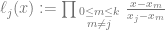
. This means that we are going to do a loop, but instead of adding the results of the loop, we are going to multiply them together. Where a capital sigma means sum, capital pi means product.

The notation for product is a bit different here than in the sigma though which may be a bit tricky to read at first. Instead of explicitly saying that m should go from 0 to k, the notation $latex 0\le m\le k\\$ says that implicitly. That same notation can be used with sigma, or the more explicit style notation could be used with pi.

The pi also has this notation next to it m\neq j. That means that the case where m equals j should be skipped.

Finally, on to the second part: \frac{x-x_m}{x_j-x_m}. This part is pretty easy to read. x is the parameter to the function of course, x_m is just controlPoints[m].x where m is the index variable of our product loop (\prod), and x_j is just controlPoints[j].x where j is the index variable of our summation loop (\sum).

Let’s say that k was 2 because we had 3 data pairs. Our three basis functions would be:

\ell_0(x) := \frac{x-x_1}{x_0-x_1} * \frac{x-x_2}{x_0-x_2}
\ell_1(x) := \frac{x-x_0}{x_1-x_0} * \frac{x-x_2}{x_1-x_2}
\ell_2(x) := \frac{x-x_0}{x_2-x_0} * \frac{x-x_1}{x_2-x_1}

Which means that our final Lagrange interpolation function would be:

L(x) := y_0 * \frac{x-x_1}{x_0-x_1} * \frac{x-x_2}{x_0-x_2} + y_1 * \frac{x-x_0}{x_1-x_0} * \frac{x-x_2}{x_1-x_2} + y_2 * \frac{x-x_0}{x_2-x_0} * \frac{x-x_1}{x_2-x_1}

That is quite a mouth full, but hopefully you understand how we came up with that!

x_i is just controlPoints[i].x and y_i is just controlPoints[i].y.

Math Intuition

The intuition here is that we need to come up with a set of functions to multiply each control point by, such that when the function’s x value is at the control point’s x value, the function should evaluate to 1. When the function’s x value is at a different control points x value, the function should evaluate to 0. The rest of the time, the function can evaluate to whatever it wants, although again, having it have smooth values is nice to making a good curve.

So the first problem is, how do we make a function evaluate to 0 when x is at a different control point?

The easy way would be to multiply a bunch of terms together of this form (x - x_i), but make sure and not include the x of the actual control point that we are multiplying against.
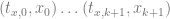
That is exactly what it does with the numerator in the product notation of the basis function.

\ell_j(x) := \prod_{\begin{smallmatrix}0\le m\le k\\ m\neq j\end{smallmatrix}} \frac{x-x_m}{x_j-x_m}

Note that j is the index of the current control point that we are calculating the basis function for. All values of x, that isn’t the x value of a control point will evaluate to non zero.

The denominator value is there so that when x is the value of the control point that we care about, that the function will evaluate to 1.

It does this by figuring out what the value of the numerator will be when x is at the control point, and then makes that be the value that it divides by, so that it’s 1 at that x value.

Not too much to it. Pretty simple stuff, but powerful as well!

Extending to 2D and Beyond

Lagrange interpolation is a one dimensional interpolation scheme, meaning that if you have data points of the form (x,y), it can give you an interpolated y value based on an x value you give it. The interpolation it does can never give two different y values for the same x.

If you want to extend this technique to interpolating a curve through two dimensional data points, or even higher, you need to do interpolation independently for each axis and use a “parametric” value for that axis.

For instance, if you needed to interpolate a curve through 3 dimensional points, you would have data points like this:

X Points = (t_{x,0}, x_0)\ldots(t_{x,k+1}, x_{k+1})
Y Points = (t_{y,0}, y_0)\ldots(t_{y,k+1}, y_{k+1})
Z Points = (t_{z,0}, z_0)\ldots(t_{z,k+1}, y_{k+1})

And then you would interpolate on each axis by the t value to get your X, Y and Z axis values. This should look familiar, because this is how higher dimensional Bezier curves work; you evaluate them per axis based on a parametric value per axis (s,t,u,etc).

You could use the same t values on each axis, or they could be completely independent. You don’t even need to have the same number of points for each axis!

You might wonder how this differs from the standard interpolation in the 2D case. Check the demos in the link section below to really get a grasp of the difference, but in essence, with standard (1D) interpolation, you can never have two x values that evaluate to 2 different y values. Extending it like the above into two dimensions by parameterizing each axis lets you get around that limitation and you can make true 2d shapes.

Lastly, it is possible to make Lagrange interpolated surfaces! I won’t go into the details (perhaps a future post!), but if you know how to make a bezier rectangle by doing a tensor product (basically having X axis Bezier curves, multiplied by Y axis Bezier curves), you can accomplish a Lagrange surface in a really similar way.

Sample Code

This sample code is written for readability, but could easily be optimized for faster execution. Also, from what I hear, the second form of Barycentric Lagrange Interpolation is touted as the fastest form of Lagrange interpolation, since many values can be pre-calculated and re-used for different values of x.

#include <stdio.h>
#include <vector>

struct SPoint
{
    float x;
    float y;
};

typedef std::vector<SPoint> TPointList;

void WaitForEnter ()
{
    printf("Press Enter to quit");
    fflush(stdin);
    getchar();
}

// calculates the lagrange basis function y value for control point "controlPointIndex" at x value "x"
float LagrangeBasis (const TPointList& pointList, size_t controlPointIndex, float x)
{
    // this is the pi "inner loop" multiplication work
    float value = 1.0f;
    for (size_t i = 0, c = pointList.size(); i < c; ++i) {
        if (i != controlPointIndex)
            value *= (x - pointList[i].x) / (pointList[controlPointIndex].x - pointList[i].x);
    }
    return value;
}

// returns a value at x, using lagrange interpolation over the specified list of (x,y) pairs
float LagrangeInterpolate (const TPointList& pointList, float x)
{
    // this is the sigma "outer loop" summation work
    float sum = 0.0f;
    for (size_t controlPointIndex = 0, c = pointList.size(); controlPointIndex < c; ++controlPointIndex)
        sum += pointList[controlPointIndex].y * LagrangeBasis(pointList, controlPointIndex, x);
    return sum;
}

int main (int argc, char **argv)
{
    // show some 1d interpolated values
    // note that the points don't need to be sorted on X, but it makes for easier to read examples
    {
        // (x,y) pairs
        const TPointList points =
        {
            { 0.0f, 1.1f },
            { 1.6f, 8.3f },
            { 2.3f, 6.5f },
            { 3.5f, 4.7f },
            { 4.3f, 3.1f },
            { 5.9f, 7.5f },
            { 6.8f, 0.0f }
        };

        // show values interpolated from x = 0, to x = max x
        printf("1d interpolated values.  y = L(t)n");
        const float c_numPoints = 10;
        for (int i = 0; i < c_numPoints; ++i)
        {
            float percent = ((float)i) / (float(c_numPoints - 1));
            float x = points.back().x * percent;
            float y = LagrangeInterpolate(points, x);
            printf("  (%0.2f, %0.2f)n", x, y);
        }
        printf("n");
    }

    // show some 2d interpolated values
    // also note that x and y don't have to have matching t values!
    {
        // (t, x) pairs
        const TPointList pointsX =
        {
            { 0.0, 0.0f},
            { 1.0, 1.6f},
            { 2.0, 2.3f},
            { 3.0, 3.5f},
            { 4.0, 4.3f},
            { 5.0, 5.9f},
            { 6.0, 6.8f}

        };
        // (t, y) pairs
        const TPointList pointsY =
        {
            { 0.0f, 1.1f },
            { 1.0f, 8.3f },
            { 2.0f, 6.5f },
            { 3.0f, 4.7f },
            { 4.0f, 3.1f },
            { 5.0f, 7.5f },
            { 6.0f, 0.0f }
        };

        // show values interpolated from t = 0, to t = max t, on each axis
        printf("2d interpolated values.  x = L(t_x), y = L(t_y)n");
        const float c_numPoints = 10;
        for (int i = 0; i < c_numPoints; ++i)
        {
            float percent = ((float)i) / (float(c_numPoints - 1));

            // calculate x
            float tx = pointsX.back().x * percent;
            float x = LagrangeInterpolate(pointsX, tx);

            // calculate y
            float ty = pointsY.back().x * percent;
            float y = LagrangeInterpolate(pointsY, ty);

            printf("  (%0.2f, %0.2f)n", x, y);
        }
        printf("n");
    }

    WaitForEnter();
    return 0;
}

And here’s the programs output:

Final Notes

Now that you know how to do all this stuff I wanted to share a couple more pieces of info.

Firstly, it’s kind of weird to call this “Lagrange Interpolation”. A better term is to call this the “Lagrange Form of Polynomial Interpolation”. The reason for that is that if you have some number of data points, there exists only one unique minimal order polynomial (lowest degree of x possible) that fits those points. That is due to the “unisolvence theorem” that you can read more about here: Wikipedia: Polynomial interpolation.

What that means is that if you were to use a different type of polynomial interpolation – such as newton interpolation – the result you get out is algebraically equivalent to the one you’d get from this Lagrange form. There are pros and cons to using different forms of polynomials, but that’s out of the scope of this post so go read about them if you are interested!

Speaking of that, even though this sample code is focused on interpolation using the Lagrange form, this technique is really great at being able to just come up with some simpler f(x) function that passes through specific data points. In this way, you can kind of “bake out” a custom f(x) function to do interpolation for specific values, that doesn’t need all the moving parts of the Lagrange form. For example, if you make the formula for lagrange interpolation of 3 specific value pairs and then simplify, will get out a simple quadratic function in the form of y=Ax^2+Bx+C!

Links

Here are some interactive demos I made to let you play with Lagrange interpolation to get a feel for how it works, and it’s strengths and weaknesses:
One Dimensional Lagrange Interpolation
Two Dimensional Lagrange Interpolation

I also found these links really helpful in finally understanding this topic:
Lagrange Interpolation
Lagrange’s Interpolation Formula

Want to follow the rabbit hole a little deeper? Check out how sinc interpolation relates to the Lagrange form!
The ryg blog: sinc and Polynomial interpolation

The De Casteljau Algorithm for Evaluating Bezier Curves

Over the past year or so I’ve been digging fairly deeply into curves, mostly into Bezier curves specifically.

While digging around, I’ve found many mentions of the De Casteljau algorithm for evaluating Bezier curves, but never much in the way of a formal definition of what the algorithm actually is, or practical examples of it working.

Now that I understand the De Casteljau algorithm, I want to share it with you folks, and help there be more useful google search results for it.

The De Casteljau algorithm is more numerically stable than evaluating Bernstein polynomials, but it is slower. Which method of evaluating Bezier curves is more appropriate is based on your specific usage case, so it’s important to know both.

If you are looking for the mathematical equation of a Bezier curve (the Bernstein form which uses Bernstein basis functions), you have come to the right place, but the wrong page! You can find that information here: Easy Binomial Expansion & Bezier Curve Formulas

Onto the algorithm!

The De Casteljau Algorithm

The De Casteljau algorithm is actually pretty simple. If you know how to do a linear interpolation between two values, you have basically everything you need to be able to do this thing.

In short, the algorithm to evaluate a Bezier curve of any order N is to just linearly interpolate between two curves of degree N-1. Below are some examples to help show some details.

The simplest version of a Bezier curve is a linear curve, which has a degree of 1. It is just a linear interpolation between two points A and B at time t, where t is a value from 0 to 1. When t has a value of 0, you will get point A. When t has a value of 1, you will get point B. For values of t between 0 and 1, you will get points along the line between A and B.

The equation for this is super simple and something you’ve probably seen before: P(t) = A*(1-t) + B*t.

The next simplest version of a Bezier curve is a quadratic curve, which has a degree of 2 and control points A,B,C. A quadratic curve is just a linear interpolation between two curves of degree 1 (aka linear curves). Specifically, you take a linear interpolation between A,B, and a linear interpolation between B,C, and then take a linear interpolation between those two results. That will give you your quadratic curve.

The next version is a cubic curve which has a degree of 3 and control points A,B,C,D. A cubic curve is just a linear interpolation between two quadratic curves. Specifically, the first quadratic curve is defined by control points A,B,C and the second quadratic curve is defined by control points B,C,D.

The next version is a quartic curve, which has a degree of 4 and control points A,B,C,D,E. A quartic curve is just a linear interpolation between two cubic curves. The first cubic curve is defined by control points A,B,C,D and the second cubic curve is defined by control points B,C,D,E.

So yeah, an order N Bezier curve is made by linear interpolating between two Bezier curves of order N-1.

Redundancies

While simple, the De Casteljau has some redundancies in it, which is the reason that it is usually slower to calculate than the Bernstein form. The diagram below shows how a quartic curve with control points A,B,C,D,E is calculated via the De Casteljau algorithm.

Compare that to the Bernstein form (where s is just (1-t))

P(t) = A*s^4 + B*4s^3t + C*6s^2t^2 + D*4st^3 + E*t^4

The Bernstein form removes the redundancies and gives you the values you want with the least amount of moving parts, but it comes at the cost of math operations that can give you less precision in practice, versus the tree of lerps (linear interpolations).

Sample Code

Pretty animations and intuitive explanations are all well and good, but here’s some C++ code to help really drive home how simple this is.

#include <stdio.h>

void WaitForEnter()
{
    printf("Press Enter to quit");
    fflush(stdin);
    getchar();
}

float mix(float a, float b, float t)
{
    // degree 1
    return a * (1.0f - t) + b*t;
}

float BezierQuadratic(float A, float B, float C, float t)
{
    // degree 2
    float AB = mix(A, B, t);
    float BC = mix(B, C, t);
    return mix(AB, BC, t);
}

float BezierCubic(float A, float B, float C, float D, float t)
{
    // degree 3
    float ABC = BezierQuadratic(A, B, C, t);
    float BCD = BezierQuadratic(B, C, D, t);
    return mix(ABC, BCD, t);
}

float BezierQuartic(float A, float B, float C, float D, float E, float t)
{
    // degree 4
    float ABCD = BezierCubic(A, B, C, D, t);
    float BCDE = BezierCubic(B, C, D, E, t);
    return mix(ABCD, BCDE, t);
}

float BezierQuintic(float A, float B, float C, float D, float E, float F, float t)
{
    // degree 5
    float ABCDE = BezierQuartic(A, B, C, D, E, t);
    float BCDEF = BezierQuartic(B, C, D, E, F, t);
    return mix(ABCDE, BCDEF, t);
}

float BezierSextic(float A, float B, float C, float D, float E, float F, float G, float t)
{
    // degree 6
    float ABCDEF = BezierQuintic(A, B, C, D, E, F, t);
    float BCDEFG = BezierQuintic(B, C, D, E, F, G, t);
    return mix(ABCDEF, BCDEFG, t);
}

int main(int argc, char **argv)
{
    struct SPoint
    {
        float x;
        float y;
    };

    SPoint controlPoints[7] =
    {
        { 0.0f, 1.1f },
        { 2.0f, 8.3f },
        { 0.5f, 6.5f },
        { 5.1f, 4.7f },
        { 3.3f, 3.1f },
        { 1.4f, 7.5f },
        { 2.1f, 0.0f },
    };

    //calculate some points on a sextic curve!
    const float c_numPoints = 10;
    for (int i = 0; i < c_numPoints; ++i)
    {
        float t = ((float)i) / (float(c_numPoints - 1));
        SPoint p;
        p.x = BezierSextic(controlPoints[0].x, controlPoints[1].x, controlPoints[2].x, controlPoints[3].x, controlPoints[4].x, controlPoints[5].x, controlPoints[6].x, t);
        p.y = BezierSextic(controlPoints[0].y, controlPoints[1].y, controlPoints[2].y, controlPoints[3].y, controlPoints[4].y, controlPoints[5].y, controlPoints[6].y, t);
        printf("point at time %0.2f = (%0.2f, %0.2f)n", t, p.x, p.y);
    }

    WaitForEnter();
}

Here’s the output of the program:

Thanks to wikipedia for the awesome Bezier animations! Wikipedia: Bézier curve

What is Pre-multiplied Alpha and Why Does it Matter?

The usual equation for blending two pixels with alpha is to use a source factor of “source alpha” and a destination factor of “one minus source alpha”.

That results in this equation:

\bf{Out.RGB} = In.RGB * In.A + Out.RGB * (1.0 - In.A)

In other words, it’s just a linear interpolation between In and Out, using the alpha of the pixel you are writing to determine the weighting for the lerp.

Just to be clear, Out is the pixel in your frame buffer (ie the final result that shows up on your monitor) and In is the new pixel you are trying to write or combine with the output image.

If you use pre-multiplied alpha, all that means is that In.RGB is already multipled by In.A which results in slightly less math:

\bf{Out.RGB} = In.RGB + Out.RGB * (1.0 - In.A)

Less math for the same results is always a good thing due to increased efficiency, but this also results in a higher quality results in the case of using mips. For more info on that check out this link: NVIDIA GameWorks – Alpha Blending: To Pre or Not To Pre

To achieve this in OpenGL or DirectX with pre-multiplied alpha textures, you just use a source factor of “one” and leave the destination factor at “one minus source alpha”.

If you are using alpha to write to a render target that also has an alpha channel, the math improvement is even better. Here is the equation with regular (post-multiplied) alpha in that scenario for combining the RGB portion of the pixels:

\bf{Out.RGB} = \frac{In.RGB * In.A + Out.RGB * Out.A * (1.0 - In.A)}{In.A + (1.0 - In.A) * Out.A}

When working with pre-multiplied alpha it just goes back to the lerp:

\bf{Out.RGB} = In.RGB + Out.RGB * (1.0 - In.A)

When blending to a target with alpha, the equation to combine alpha is the old familiar lerp:

\bf{Out.A} = In.A + Out.A * (1.0 - In.A)

That makes the lerp form of color combining even nicer since it means the same math for all color channels of the pixel:

\bf{Out} = In + Out * (1.0 - In.A)

Confused about why alpha combining using lerp makes sense? It makes most sense to me when thinking about it like this… if you had something that was half opaque(Out.A = 0.5), then you looked at that through something that was 3/4 opaque (In.A = 0.75), only 25% of the light would get past the top layer (0.25), to reach the bottom layer. Only 50% of the light that reached the bottom layer gets through, so we cut that 25% in half to get 12.5% (0.125). Since alpha really means “opaqueness” (1.0 means no transparency), that means that the combined alpha is 1 – 0.125, or 0.875.

If you plug the numbers into the above equation you get the same result:

\bf{Out.A} = 0.75 + (1.0 - 0.75) * 0.5
\bf{Out.A} = 0.75 + 0.25 * 0.5
\bf{Out.A} = 0.75 + 0.125
\bf{Out.A} = 0.875

This compute graphics stack exchange question has some more great info on what premultiplied alpha can give you. It’s much more than I wrote here:
Does premultiplied alpha give order independent transparency?

Here’s a fun question… does alpha represent transparency, or does it represent how much of a pixel is covered by an opaque object? To find out the answer give this a read!
Jounral of Computer Graphics Techniques: Interpreting Alpha

Adventures in Learning How to Publish a Research Paper Part 1

So I’m in the process of trying to get a research paper published and wanted to share what I’ve learned so far. I’ll continue to write more beyond this post as I continue the process. Yes, I know my writing is terrible (grammar etc), please don’t take this as a representation of the final product 😛

The world of published papers, journals and academia (not necessarily lumped into the same group) is a bit different than I expected. On the whole, I’ve found that it’s both more approachable than I expected, and less approachable than I expected, in different, unexpected ways.

Motivation

A handful of times in my life, I’ve come up with things, naiively thought that I had invented it, and then later found out that it already existed and was a known thing.

I’ve reached the point in my career and personal growth where I’m coming up with things that seem like finally, they may not actually yet be already known and exist.

A braver person may quit their job and start a software company and try to make it happen and then possibly fail 9 out of 10 attempts (hey look, im about to cite something that refutes that statement Washington Post: Do nine out of 10 new businesses fail, as Rand Paul claims?).

Maybe a more cunning, yet less adventurous person would try and patent their idea, then sell the patent, or wait for someone to intrude and then sue for damages. I don’t like the idea of patenting my ideas or techniques because honestly, I want other people to do things with them, I just want to be the first, and I want people to know I was the first (petty perhaps but at least I’m being honest haha).

I happen to be taking perhaps the least risky road, but seemingly most altruistic path (more info on that later), and am thinking about publishing my techniques in a research journal of an appropriate field. This way, everyone is free to use it, and I can see what other people do with it – if anything. I will be known as “the guy who came up with this”, but probably won’t ever actually get to use it in my actual job. Boo-hoo! (we’ll see I guess…)

You never know though… having published papers definitely ought to lead to better career advancement opportunities, and frankly, maybe some dream job will come along where I get to work on these topics I’m publishing about, and do some cutting edge research towards practical results, and push the envelope of what people think can be achieved with current technology. That would be pretty cool! If you are a game (or related) company that is heavy in research, and also practical results, working within the realm of real time raytracing, unorthodox graphics techniques, VR, and other cool tech, and interested in a dude such as myself, drop me a line. I’m happy where I am but never hurts to chat and network (;

Anyhow, with a 1 year old baby, a house payment, and the like, I need the stability. I can’t go starting a new company so a research paper it is!

A quick note to my son Loki, if he reads this in the future, a nice little time capsul for him 😛

Hello Loki! I love you very much and I hope you are doing well. Your initials are LZW which is a compression algorithm, and your namesake is the norse god of mischief. Your mom is a super smart psychologist, so I hope we’ve taught you well and that you are now a Robot Psychologist AI developer who somehow furthered the works of chaos theory for AI and data compression. Or… you can play guitar at starbucks. Whatever makes you happy (: Talk to you later – dad. PS bring me a beer pls!!

Misconceptions Untangled

Once the decision of publishing in a journal was made… it was time to figure out what the heck academia / research papers were all about. As a near high school drop out with no degree, all I really know is what my near PHd wife (educational psychology) and more educated friends and family have told me.

Here were some of my misconceptions when I started out:

  • Publishing a paper is not for the likes of a mere mortal like me
  • When a paper makes a statement backed by a reference to something else that says so, that is irrefutable evidence that it is fact.
  • Publishing papers is all about advancing science, and perhaps a bit about one’s ego, but not at all about money
  • When you publish something, it has to be new. In fact, it has to be so novel that it can’t be like anything else written EVER.
  • Google ought to be great at helping me find other related work that i can reference!

Let’s address these points.

Publishing a paper is not for the likes of a mere mortal like me

Yes it is. Flat out, it is for anyone who wants to participate.

YOU have something to contribute to the world, but even moreso, writing and publishing a paper isn’t as impressive as it may sound. That thought will be continued below.

When a paper makes a statement backed by a reference to something else that says so, that is irrefutable evidence that it is fact

Wrong! At best, all that means is that someone else said the same thing. At worst, it means that they misinterpreted the thing they cited.

In either case, it’s through “peer review” that we hope mistakes and fallacies are found and corrected before publication, but it’s all humans involved, and humans are imperfect machines.

This is likely basic info for anyone who went to college, but for the rest of us simple folk, this translates to: Check your sources, and make sure you have multiple sources that are in agreement. Also try to understand and address any source that disagrees.

Publishing papers is all about advancing science, and perhaps a bit about one’s ego, but not at all about money

Sure it is about advancing science, and perhaps a bit about one’s ego, but there is more to it.

Certain professions are bound as part of their employment contract to fulfill a quota of published papers. Kind of surprising isn’t it?

Also, it costs MONEY to submit papers to journals. Like 5 grand or more. Where does that money go? You’d hope it would go to fund other research, but I’m not really sure where it goes in general. It also varies from journal to journal.

Furthermore, it costs money to READ papers in journals. Yes, seriously. Someone did science for the benefit of the world, and wanted to put it out there for the world to see and make use of, and the journals charge quite a bit of money to anyone who wants to read these papers. In practice, only academic institutions likely have access to these papers.

Are you an independent researcher with something to share with the world? Too bad! Good luck even finding related work to cite or improve upon jerk! ha ha ha!

Basically, academic journals are there for academic folk to publish in, get well known in academic circles, get better academic jobs and kinda stay in that realm.

Similarly, those folks aren’t likely to show things at E3.

It’s just a different world with it’s own rules and people in that system have different goals than us folk developing video games or graphics applications.

When you publish something, it has to be new. In fact, it has to be so novel that it can’t be like anything else written EVER.

Funny enough, it turns out this doesn’t have to be true at all.

If you are patenting an idea, you need to look like it came from NO WHERE and that it’s the first of it’s kind and is super amazing and standalone.

If you are publishing a paper, it’s kinda the reverse that is true. To gain credibility you need to show how your work is based on work other folks have done, and how you’ve improved them.

Alternately, you could also just do a paper that is a survey of various techniques to show the pros and cons of each.

Lastly, you can even write about something someone else already wrote about, but just explain it better, or maybe explore some of the implications of their work that they didn’t.

Yeah. YOU right now, could write a research paper about something. I guarantee you could. It just will take some time and effort (and possibly money), which may or may not be worth it to you.

Google ought to be great at helping me find other related work that i can reference!

This is still a bit strange to me. Google has been NO help in finding work related to what I’ve been working on.

On one hand, I can see that being true due to research almost always being behind a pay wall that google can’t see behind, but on the other hand, there is a lot of research that isn’t. Also, the “Abstract” of papers (a ~4 sentence summary) is almost always able to be read for free. Why does google not have knowledge of those?

But yeah… google has found NOTHING. The references I have are things that I accidentally stumbled on, or that other people RANDOMLY happened to put something on twitter about, or talk about in graphics mailing lists.

I search for exact terms that should find things I now know exist, and it finds nothing.

WTF Google?!

Is it Worth it?

As a (professional?) (game?) programmer, is publishing a paper worth it? It depends.

Is this something you have a desire to do? I have always wanted to be a scientist and contribute to human progress, so that makes it worth while to me.

Also, it can’t hurt the resume, but it can be expensive.

If interested, make sure and find out what your employer’s policies are though, and also what your rights are which may be different than what your company would like you to do!

Then, in the end, do whatever you think is best (:

It’s also a good idea to read the guidelines for submission from the journal, read the notes that they give to reviewers to help review your paper, and also you should read papers that have been published in that journal to get an idea of what qualities an accepted paper has.

Some Resources

Here are some nice resources I’ve found so far.

First and foremost is the journal I’m going to be trying to publish my first paper with. They have some sort of partnership with SIGGRAPH which is awesome (because SIGGRAPH is amazing!!), and also, it’s FREE to submit papers to, and FREE for people to read. It’s also aimed towards professional game / graphics programmers and focuses more on practicality and results, and less on purely theoretical things, or typical academic practices that don’t really have a place in the non academic world (IMO). Go right now and go read some of their articles!

http://jcgt.org/ – the Journal ofComputer Graphics Techniquespeer-reviewed, open access, and free to all

Next, I encourage you to read the notes that jcgt gives to reviewers to help them review papers. This ought to show you the mindset of both the journal and the reviewers. They are literally there to try and help you succeed as much as possible.

JCGT – Review Form

I also want to share this presentation with you, which is from Microsoft Research, Cambridge.

How to write a great research paper

If you are someone like me who wishes for greatness, but feels like a “mere mortal”, I really recomend reading the book “Masters of Doom” to see how John Carmack and related folk made such a splash in the world as game developers. JC is someone I respect a lot, and a lot of things he does and has done in the past are things that are beyond my wildest dreams of success, but things I’d like to aspire to. The path is a lot more humble than you might expect, and even a little bit shady at times. Masters of Doom: How Two Guys Created an Empire and Transformed Pop Culture.

Lastly, as I write my paper, I hope that this is the time that I finally have invented something that doesn’t yet exist (please???!!!). I’ve spent several months on doing experiments, writing code, doing research to help explain my results, and finding ways to work around problems encountered. I’ve finally finished that phase and have started in on actually writing the paper (abstract v1 is finished, outline is work in progress).

RANDOMLY, last friday, someone posted a link to a paper in a graphics mailing list I’m on. That paper had a title so similar to what I’m writing that i nearly fell out of my chair and started crying LOL (ok maybe exaggerating but i was scared). I read it in a few passes, each time peeking out from between my fingers as i was covering my eyes, afraid of what I’d see, and after about 4 or 5 of those passes I gave a sigh of relief. There are similarities, but it is a world of different-ness, and it’s applications are way different than my paper.

PHEW. That close call actually gave me the strongest reference I have to cite and actually gave me some references to other papers which explain some of the strange results I was getting in a specific situation, so solved a mystery for me. Turned out to be a good thing, but man was I scared.

Believe it or not, the academia stack exchange site has been a great help too in finding answers to specific questions that you can’t just ask google about:
https://academia.stackexchange.com/

More coming in the future as I learn more, until then, ta ta!

A Fifth Way to Calculate Sine Without Trig

In a previous post, I showed Four Ways to Calculate Sine Without Trig. While reading up on rational bezier curves, I came across a 5th way!

A rational bezier curve post will be coming in the (hopefully near) future, so I won’t go into too many details of that, but the important thing to know is that with a rational 2d quadratic bezier curve, you can EXACTLY represent any conic section, including circle arcs. With a regular (integral) bezier curve, you can’t.

You can in fact see that in action in an interactive HTML5 demo i made here: Rational Quadratic Bezier Curve. Note that on my main page, i have links to other 1d/2d bezier/trig rational/integral interactive curve demos. go check them out if you are interested in seeing more: http://demofox.og.

After I made the 2d quadratic bezier demo I realized something… The x and y positions of that curve are calculated independently of each other, and if you wanted to draw a circle in a program, you’d calculate the x and y positions independently, using sine for the y axis value and cosine for the x axis value. That means that if rational curves can – as people say – perfectly represent conic sections, that the two 1d curves that control each axis of that circle arc curve must be exact representations of sine and cosine, at least for the 90 degrees of that arc.

It turns out that this is true enough. I am seeing some variation, but have an open question on math stack exchange to try to get to the bottom of that.

Let’s do some math to come up with our curve based sine equation!

Math Derivation – Skip If You Want To

A rational Bezier equation is defined like this, which is basically just one Bezier curve divided by another:

\bf{B}(t) = \frac{\sum\limits_{i=0}^n\binom {n} {i}(1-t)^{n-i}t^iW_iP_i}{\sum\limits_{i=0}^n\binom {n} {i}(1-t)^{n-i}t^iW_i}

So, here is the equation for a rational quadratic bezier curve (n = 2):

\bf{B}(t) = \frac{(A*W_1*(1-t)^2 + B*W_2*2t(1-t) + C*W_3*t^2)}{(W_1*(1-t)^2 + W_2*2t(1-t) + W_3*t^2)}

A,B,C are the control points and W_1,W_2,W_3 are the weightings associated with those control points.

For the first 90 degrees of sine, A=0, B=1, C = 1, W_1 = 1, W_2 = cos(arcAngle/2), W_3 = 1.

arcAngle is 90 degrees in our case, so W_2=cos(45) or W_2=1/sqrt(2) or W_2=0.70710678118.

If we plug those values in and simplify, and treat it as an explicit (1d) equation of y = f(x), instead of P=f(t), we come up with the equation in the next section.

Final Equation

y = \frac{(0.70710678118*2x(1-x) + x^2)}{((1-x)^2 + 0.70710678118*2x(1-x) + x^2)}

or, so you can copy paste it:
y=(0.70710678118*2x(1-x) + x^2) / ((1-x)^2 + 0.70710678118*2x(1-x) + x^2)

That gives us the first quadrant (first 90 degrees) of sine. To get the second quadrant, we just horizontally flip the first quadrant. To get the third quadrant, we vertically flip the first quadrant. To get the fourth quadrant, we vertically and horizontally flip the first quadrant.

Equation In Action

Here’s a screenshot from a shadertoy where I implemented this. red = true sine value, green = the value made with the curve, yellow = where they overlap and are equal. Any place you see red or green peaking out means they aren’t quite equal. I sort of expected it to be exactly dead on correct, but like I said, I have an open math stack exchange question to find out why it isn’t and will update this with my findings if they are relevant or interesting. It still is pretty darn good though.

Also, this formula may not be the most efficient way to calculate sine without trig that I’ve shown, but it is interesting, and that’s why I wanted to show it (:

You can see this in action at Shadertoy: Sin Without Trig IV

Easy Binomial Expansion & Bezier Curve Formulas

In this post we are going to explore two things:

  1. Learn how to easily be able to expand (x+y)^N for ANY value N using the binomial theorem (well, N has to be a positive integer…)
  2. Use that for coming up with the equation for a Bezier curve of any degree (any number of control points)

Binomial Theorem

The binomial theorem is a way of easily expanding (x+y)^N. As you probably know, if N is 2, you can use FOIL (first, outer, inner, last). If N gets above 2, things start to get harrier though and more tedious.

Let’s check out how the values look when N is 1, 2 and 3:

N (x+y)^N Expanded
1 x+y
2 x^2+2xy+y^2
3 x^3+3x^2y+3xy^2+y^3

To help make the patterns more visible, let’s make things a bit more explicit:

N (x+y)^N Expanded
1 1x^1y^0+1x^0y^1
2 1x^2y^0+2x^1y^1+1x^0y^2
3 1x^3y^0+3x^2y^1+3x^1y^2+1x^0y^3

The easiest pattern to see is that there are N+1 terms.

The next pattern that might jump out at you looking at the above table, is that in the first term, y starts out at power 0, and the next term has a power of 1, and the power of y keeps increasing by 1 for each term left to right until we run out of terms. Similarly, x starts out at a power of 0 on the last term, has a power of 1 on the second last term, and counts up going from right to left, until we run out of terms.

Those patterns explain how many terms there are and the powers of x and y for each term. There is one piece left of the puzzle though, which is those constants that each term is multiplied by.

Those constants are called the “binomial coefficients” and they also appear as rows on pascal’s triangle. In short, each number in pascal’s triangle is a sum of the numbers directly above it. Below is an image to show what I’m talking about. Check the links section at the end for more detailed info.

So if you notice, the 2nd row of pascal’s triangle is “1,1”. Those are the constants multiplied by each term for the N=1 case. The next row down is “1,2,1” which is the constants multiplied by each term for the N=2 case. Lastly the next row down (fourth row) is “1,3,3,1” which is the constants multiplied by each term for the N=3 case. Essentially, you just use the N+1th tow of pascals triangle to come up with the constants to multiply each term by.

There are algorithms for calculating the N+1th row of the pascal’s triangle. I have one such algorithm in the example code below, but also check the links section for more info on that.

TADA! That is the binomial theorem.

Bezier Curve Equation Generalized (Again)

You may remember that I previously showed you a generalized way to get the equation for a bezier curve of any order in Bezier Curves Part 2 (and Bezier Surfaces).

It wasn’t too difficult, but it DID require you to manually expand (x+y)^N. Now that we know how to do that more easily, thanks to the section above, let’s revise how we come up with bezier curves of any order.

What you do is evaluate P=(s+t)^N, and then multiply each term by a unique control point (A,B,C,etc). After you have your equation, you can optionally replace all s‘s with (1-t), or you can just remember that when you evaluate the equation, since the first form is less messy.

Boom, you are done, that’s all!

Here’s the quadratic (N=2) version to see the end result:
P = As^2 + 2Bst + Ct^2

Formalized Mathematical Description

The above makes a lot of sense and is easy to understand, wouldn’t it be neat if math could describe it that way?

Well… it turns out it can, and does. Here is the formal “explicit definition” of bezier curves:
\sum\limits_{i=0}^n\binom {n} {i}(1-t)^{n-i}t^iP_i

If you remember from above, s is the same as (1-t) so you could also write it like this:
\sum\limits_{i=0}^n\binom {n} {i}s^{n-i}t^iP_i

The \sum\limits_{i=0}^n (Sigma, going from 0 to n) means that you are going to sum (add) together n+1 terms (it includes both 0 and n), using i as the loop variable in your summation. It’s basically a for loop, adding together each iteration of the for loop. Everything that comes after is what happens during each iteration of the for loop that gets summed together.

The \binom {n} {i} part means to take the ith number from the (n+1)th row of Pascal’s triangle. More formally, this specifies to use specific binomial coefficients.

The next part s^{n-i}t^i 
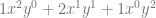
means that you multiply the binomial coefficient by s to the (n-i)th power, and t to the ith power. This is the same as saying s starts at power n and counts down left to right, while t starts at 0 and counts up left to right. This fits the pattern we saw above in binomial expansion.

Lastly comes P_i which means to use the ith P. So, P is basically an array with n+1 elements. This array is the control points, so each P is a different control point.

So, to sum it all up, it’s saying to make a for loop from 0 to n where you are going to add up the results of each for loop. For each loop iteration, where i is the index variation of the loop, you are going to:

  1. Start with the ith item from the (n+1)th row of pascals triangle
  2. Multiply that by s^(n-i)t^i
  3. Multiply that by a unique control point

There ya go, formalized math descriptions with crazy symbols can actually mean something useful. Who would have thought?!

Here is the quadratic bezier curve again for you to look at (quadratic means n = 2), in a form that will help you when thinking about the steps above:
P = 1s^2t^0A + 2s^1t^1B + 1s^0t^2C

And when it’s cleaned up, it looks more familiar:
P = As^2 + 2Bst + Ct^2

Example Code

#include <stdio.h>
#include <vector>

//=====================================================================================
void WaitForEnter ()
{
    printf("nPress Enter to quit");
    fflush(stdin);
    getchar();
}

//=====================================================================================
std::vector<unsigned int> PascalsTriangleRow(int row)
{
	std::vector<unsigned int> ret;
	ret.push_back(1);
    for (int i = 0; i < row; ++i)
        ret.push_back(ret[i] * (row - i) / (i + 1));
	return ret;
}

//=====================================================================================
void main(void)
{
	printf("Expand (x+y)^N and give Bezier curve order NnnPlease enter N:n");
	unsigned int N;
	// keeping it limited to a sane value. also protects against -1 being huge.
	// Also, so we don't run out of letters for control points!
	if (scanf("%u",&N)==1 && N < 26)
	{
		auto row = PascalsTriangleRow(N);

		// binomial expansion
		printf("nBinomial Expansion:n");
		if (N == 0)
		{
			printf("1");
		}
		else
		{
			for (unsigned int i = 0, c = row.size(); i < c; ++i)
			{
				if (i > 0)
					printf(" + ");

				if (row[i] != 1)
					printf("%u", row[i]);

				unsigned int xPow = N - i;
				if (xPow > 0)
				{
					printf("x");
					if (xPow > 1)
						printf("^%i", xPow);
				}

				unsigned int yPow = i;
				if (yPow > 0)
				{
					printf("y");
					if (yPow > 1)
						printf("^%i", yPow);
				}
			}
		}

		// bezier curves
		printf("nnBezier Curve Order %u:nP = ", N);
		if (N == 0)
		{
			printf("A");
		}
		else
		{
			for (unsigned int i = 0, c = row.size(); i < c; ++i)
			{
				if (i > 0)
					printf(" + ");

				// control point name
				printf("%c*",'A'+i);

				if (row[i] != 1)
					printf("%u", row[i]);

				unsigned int sPow = N - i;
				if (sPow > 0)
				{
					printf("s");
					if (sPow > 1)
						printf("^%i", sPow);
				}

				unsigned int tPow = i;
				if (tPow > 0)
				{
					printf("t");
					if (tPow > 1)
						printf("^%i", tPow);
				}
			}
		}

		// bezier curves
		printf("nnOr:nP = ", N);
		if (N == 0)
		{
			printf("A");
		}
		else
		{
			for (unsigned int i = 0, c = row.size(); i < c; ++i)
			{
				if (i > 0)
					printf(" + ");

				// control point name
				printf("%c*",'A'+i);

				if (row[i] != 1)
					printf("%u", row[i]);

				unsigned int sPow = N - i;
				if (sPow > 0)
				{
					printf("(1-t)");
					if (sPow > 1)
						printf("^%i", sPow);
				}

				unsigned int tPow = i;
				if (tPow > 0)
				{
					printf("t");
					if (tPow > 1)
						printf("^%i", tPow);
				}
			}
		}

		printf("n");
	}
	else
	{
		printf("Invalid value for Nn");
	}
	WaitForEnter();
}

Example Output

Here are some runs of the program


Links

Note that even though we talked about binomials, and bezier curves, these techniques can be expanded to trinomials and bezier triangles – and beyond! (hint: there is such thing as Pascal’s pyramid!)

Here are some links to more info about some of the topics talked about above:
Wikipedia: Binomial Theorem
Wikipedia: Pascal’s Triangle
Wikipedia: Binomial Coefficient
StackOverflow: How to efficiently calculate a row in pascal’s triangle?

No Bad Code, Creeping Normality and Social Structure Code Organization

In the last post I said that another post was coming regarding using bilinear texture sampling for something interesting. Hopefully without sounding too pretentious, that interesting thing I wanted to write up has shown quite a bit of fruit, so I’m going to try to write it up and see about getting it put into The Journal of Computer Graphics Techniques. We’ll see how that pans out, and I’ll make sure and share once it’s published (or if I can’t get it published hehe) as well as a post on the process of trying to get something published, in case other people out there are interested in pursuing that sort of thing.

Today’s post is a bit different than usual. There are some interesting concepts that I’ve been exposed to that I think are worth sharing, and that I’m hoping you will also find interesting.

No Bad Code

One idea presented to me recently was the concept that there is no bad code. The idea being that people make decisions in code based on the situations at the time, and that as situations change, code that once was totally reasonable, and most engineers would likely have made the same choices, no longer is seen as a good choice in the new sets of circumstances.

I’m going to be a bit cynical here and mention that I do believe there is bad code, and that it comes around due to bugs, as well as lack of knowledge, lack of experience, and lack of testing before deployment. However, the idea of code that is now seen as bad, was once perfectly reasonable does make sense to me and is kind of interesting.

I know we’ve all hit code that we or others wrote that we despise, causes us grief, and gets in the way of us working what we ought to be working on. This concept definitely does absolve SOME such code I’ve personally had to deal with. But, there is definitely plenty of code left that it doesn’t. In my personal examples, this mostly comes from shoddy third party middleware software, and also, just a lack of knowledge or experience on the part of the implementer. I’m guilty of the second point, but I think we all are, and that is a sign we are learning and growing.

It’s probably good to keep in mind that lousy code of the present may have been perfectly reasonable code of the past, and before deciding that code was lousy, or that a specific engineer is terrible, that you have to judge the code in the light that it was put in.

… Then refactor it.

Creeping Normality

Creeping normality is an interesting concept. Basically, just like that old tale of a frog sitting in progressively hotter water til it boils (which by the way is debunked by snopes), it’s easy for individuals or companies to find themselves in situations that would NEVER be seen as ideal situations, but were arrived at by incremental mis-steps – or also just a changing landscape.

This relates to the last point a bit, because it can show how the needs of a piece of code can change over time, such that looking at it as a static snapshot in time, you might wonder why it’s so complex and trying to do so many different things needlessly.

This can also happen to a company on a more global scale, and can explain some really odd, less than ideal behaviors a company might be doing, where you are pretty sure the people involved know better.

How do you fight creeping normality? Good question… but when you are able to identify some oddness or problems that come up due to it, hopefully it’s as early as possible, and hopefully the people with the power to make things right listen to you (:

Social Structure Code Organization

The last topic is kind of bizarre, but totally makes sense once you think about it. The idea is that code will match the communication structure of the teams making the code.

This is Conway’s law which says: “organizations which design systems … are constrained to produce designs which are copies of the communication structures of these organizations”. Another good quote from the wikipedia page for Conway’s law states that (paraphrased) “if you have four teams working on a compiler, you’ll end up with a four pass compiler”.

This can be seen a lot in situations where you have a game engineering team and an engine engineering team. There will be a distinct line between the code bases, based on the responsibility of the teams. If instead, you have some code where the engine and game team are the same, there will be no such line, and if you then try to split that team into being a game and engine team, it’ll take some time to draw the line between responsibilities, separate the code along those lines, and possibly do something like get the code into separate projects and possibly code repositories, which all seems like a logical choice to do when you have separate teams.

I think this also relates back to the first point about “No Bad Code”, because were someone to come into a team where the organization had recently changed, they are going to wonder why the code doesn’t have nice abstracted API layers at the boundaries, like most folks would consider logical and good practice. Perhaps too, this would be a case of creeping normality, or at least, if the project organization changed, it could be the result of a reaction AGAINST creeping normality.

In short, there are a lot of ways in which perfectly good code can go bad, and it’s probably a good idea to think about that a bit before condemning code as inherently rotten.

HOWEVER, rotten code does exist. I’d name some names, but it would probably be classified as slander, so i’ll bite my tongue. I’m sure you have plenty of examples of your own (;

Lastly, if you are responsible for crimes against code-manity in days past, either due to any of the reasons above, or because you didn’t know things you know now, or even if you were just lazy or misguidedly purposefully malicious (?!), remember this: You are not your mistakes!

OK, enough of that, next post will be on some cool programming technique, I promise 😛

Bilinear Filtering & Bilinear Interpolation

Take a look at the picture below. Can you calculate the values at points A,B and C?

There’s a technique for doing this called bilinear interpolation which extends the idea of linear interpolation into two dimensions.

To calculate bilinear interpolation, you just do linear interpolation on one axis, and then the other.

Check out these examples:

Point A
Point A has a coordinate of (0.2,0.8). Let’s start with the X axis.

Firstly, we’ll do interpolation across the top of the square on the X axis. That means we need to go 0.2 (20%) of the way from 7 to 0. That 0.2 is our x axis coordinate. To calculate that we do this:
7 + (0-7) * 0.2 = 5.6

Next, we’ll do interpolation across the bottom of the square on the X axis. So similar to above, we’ll go 0.2 (20%) of the way from 3 to 5. To calculate that we do this:
3 + (5-3) * 0.2 = 3.4

Now that we have interpolated across our X axis we need to interpolate across our Y axis. We are now going to go 0.8 (80%) of the way from our bottom value (the value of Y = 0), to our top value (the value of Y = 1). The bottom value is the bottom interpolation we did (3.4) and the top value is the top interpolation we did (5.6).

So, we need to go 0.8 (80%) of the way from 3.4 to 5.6. To calculate that we do this:
3.4 + (5.6 – 3.4) * 0.8 = 5.16

So, the value at point A is 5.16. The image below should help explain visually the process we went through.

Point B

Point B has a coordinates of (1.0,0.5).

Let’s start with the X axis interpolation again (although you could easily start with Y first if you wanted to! You’d end up with the same result).

Doing the X axis interpolation across the top, we need to go 1.0 (100%) of the way from 7 to 0. I’m sure you can guess what the answer is but here it is calculated:
7 + (0-7) * 1.0 = 0

Similarly, let’s do the X axis interpolation across the bottom. We need to go 1.0 (100%) of the way from 3 to 5.
3 + (5-3) * 1.0 = 5

Next up comes the Y axis interpolation. We need to go 0.5 (50%) of the way from 5 to 0.
5 + (0-5) * 0.5 = 2.5

There we go, the value at point B is 2.5. That should make sense too by looking at the diagram. It’s basically 1d linear interpolation between 5 and 0, and is half way between them, so intuitively, the answer 2.5 should make sense.

Point C

Point C has a coordinate of (0.8,0.2).

Once again, let’s do the X axis interpolation across the top of the box. We need to go 0.8 (80%) of the way from 7 to 0.
7 + (0-7) * 0.8 = 1.4

Then, we need to do the x axis interpolation across the bottom of the box. We need to go 0.8 (80%) of the way from 3 to 5.
3 + (5-3) * 0.8 = 4.6

Lastly, the y axis interpolation. We need to go 0.2 (20%) from 4.6 to 1.4.
4.6 + (1.4-4.6) * 0.2 = 3.96

The value of point C is 3.96

Bilinear Filtering

While bilinear interpolation is useful if you have a grid of data that you want to interpolate values within (such as a height field that represents terrain?!), where this really shines in game development is in bilinear texture filtering.

Basically, when you have a texture coordinate that doesn’t perfectly line up with the center of a pixel in the texture (because there’s a remainder), it uses the fractional part of the coordinate within that pixel to do bilinear interpolation between the 4 pixels involved to come up with the final pixel color. It does bilinear interpolation on each of the channels: Red, Green, Blue and Alpha.

The end result is pretty good! Check out the image below to see it in action on a texture that we are zoomed in too far on. The left side uses bilinear filtering, while the right side does not, and just shows you the nearest pixel.

Consequently, bilinear texture filtering has to do 4 pixel reads to be able to interpolate between them, instead of a single pixel read like when doing nearest pixel sampling. More pixel reads = more overhead, and not as cheap (computationally) to use.

Links

For some folks who are reading this, this info is pretty basic and you might be wondering why i bothered writing about it. Look to the next post for something kind of bizarre regarding bilinear filtering. This was needed as a stepping stone to the next thing I want to show you guys 😛

Wikipedia: Linear Interpolation

Wikipedia: Bilinear Interpolation

Wikipedia: Bilinear Filtering

The Dark Side of Bilinear Filtering

Check out these links for some deeper info about some shortcomings (and some workarounds) of hardware based bilinear sampling:
iq: hardware interpolation
iq: improved texture interpolation

FlipQuad & FlipTri Antialiasing

Here are the last two SSAA algorithms/sampling patterns that I wanted to share – FlipQuad and FlipTri.

FlipQuad

The last post talked about 4-Rook antialiasing which took 4 samples per pixel to do antialiasing.

Before that we talked about quincunx which was able to get 5 samples per pixel, while only rendering 2 samples per pixel. It was able to do that by sharing “corner samples” among 4 pixels.

If you combine the ideas from the last two posts, you could start with the 4-rook sampling points and push them to the edge of the pixel so that the edge samples can be shared between the pixels that share the edge.

If you do that though, you’ll actually have two samples on each edge. To solve this and keep the same number of sample points per pixel, you could flip every other pixel’s sample points.

Ta-Da! That is exactly what FlipQuad is. Check out the sampling pattern below, which shows the samples for a 2×2 grid of pixels. You’d just repeat this pattern for as many pixels as you had.

Here’s an image that shows FlipQuad in action – anti aliased on the left, regular image on the right. You can click on the image to see the shadertoy demo of it.

It works pretty well, but it is pretty blurry, especially the textures! Kind of makes sense because quincunx was blurry due to shared samples. We have ONLY shared samples in this pattern, so it’s understandable that it’s kind of blurry. There’s less unique information per pixel than in the other SSAA techniques shown so far.

This essentially is 2 samples rendered per pixel to get 4x SSAA.

ShaderToy: FlipQuad AntiAliasing

FlipTri

Flipquad worked decently, but instead of using a quad, could we use a triangle? Yes we can, check out the 2×2 pixel sampling pattern below:

Here’s an image that shows FlipTri in action – anti aliased on the left, regular image on the right. You can click on the image to see the shadertoy demo of it.

This essentially is 1.25 samples rendered per pixel to get 3x SSAA! It really doesn’t look that different to my eyes than the flipquad method, but it uses quite a fewer number of samples!

ShaderToy: FlipTri AntiAliasing

Conclusion

So basically, there’s a bunch of different ways to do SSAA style anti aliasing, even beyond the ones I showed, but in the end you are basically just taking more samples and/or sharing samples across multiple pixels to get a better resulting image.

SSAA is also a common technique in raytracing, where they will shoot multiple rays per pixel, and combine them together in this way, sometimes for things like movies, they will cast hundreds of rays per pixel! You could also just render multiple times and do one of the methods we’ve talked about in the last couple post instead of explicitly shooting multiple rays per pixel.

At SIGGRAPH 2014, someone mentioned in the “advancements in realtime rendering” talk that they used the flipquad pattern along with temporal supersampling. That made it so the 2 samples rendered per pixel was amortized across two frames and thus became one sample per pixel, which is pretty nifty. I feel like you could extend that to flip tri’s and perhaps render less than 1 sample per pixel each frame.

A big issue with implementing these in modern graphics situations is that it’s difficult to render a sample once and share it across multiple pixels. I have a way in mind involving rendering the scene a couple times with different sized buffers and offsets, but not sure yet if it’s practical. Temporal supersampling algorithms definitely seem like they could benefit from these exotic patterns more easily.

Up next I think I’m going to try and figure out MSAA, which has similar results as SSAA, but from the sound of things, performs a bit better.

Links

FlipQuad Research Paper: FLIPQUAD: Low-Cost Multisampling
Rasterization

FlipTri Research Paper: An Extremely Inexpensive
Multisampling Scheme

A Weighted Error Metric and Optimization Method for
Antialiasing Patterns

CGT 511
(Anti)aliasing

Bart Wronski: Temporal supersampling and antialiasing

A Family of Inexpensive Sampling Schemes