This is an extension of a paper I wrote which shows how to use the linear texture sampling capabilities of the GPU to calculate points on Bezier curves (also just polynomials in general as well as rational polynomials, and also surfaces and volumes made by tensor products). You store the control points in the texture, then sample along the texture’s diagonal to get points on the curve:
GPU Texture Sampler Bezier Curve Evaluation
This extension improves on the efficiency of the storage space usage, allowing a higher density of curve data per pixel, but the post also talks about some caveats and limitations.
This post is divided into the following sections:
- Basic Idea of Extension
- 2D Texture / Quadratic Piecewise Curves
- 2D Texture / Quadratic Piecewise Curves – C0 Continuity
- 2D Texture / Quadratic Piecewise Curves – Storage Efficiency
- Real World Limitations
- 3D Texture / Cubic Piecewise Curves
- 3D Texture / Cubic Piecewise Curves – Multiple Curves?
- 3D Texture / Cubic Piecewise Curves – C0 Continuity
- 3D Texture / Cubic Piecewise Curves – Storage Efficiency
- Generalizing The Unit Hyper Cube
- Closing
- Code
1. Basic Idea of Extension
Let’s talk about the base technique before going into the details of the extension.
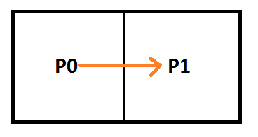
The image below shows how bilinear interpolation across the diagonal between pixels can calculate points on curves. Bilinear interpolation is exactly equivalent to the De Casteljau algorithm when the u and v coordinate are the same value.

Linear interpolation between two values A and B at time t is done with this formula:

I’ve found useful to replace (1-t) with it’s own symbol s. That makes it become this:

Now, if you bilinear interpolate between 4 values, you have two rows. One row has A,B in it and the other row has C,D in it. To bilinear interpolate between these four values at time (t,t), the formula is this:

If you expand that and collect like terms you come up with this equation:

At this point, the last step is to make B and C the same value (make them both into B) and then rename D to C since that letter is unused. The resulting formula turns out to be the formula for a quadratic Bezier curve. This shows that mathematically, bilinear interpolation can be made to be mathematically the same as the quadratic Bezier formula. (Note: there are extensions to get higher order curves and surfaces as well)
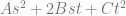
However, for this extension we are going to take one step back to the prior equation:
What you may notice is that the two values in the corners of the 2×2 bilinear interpolation don’t have to be the exact value of the middle control point of the quadratic Bezier curve – they only have to AVERAGE to that value.
This is interesting because to encode two different piecewise quadratic curves (C0-C2 and C3-C5) into a 2d texture before this extension, I would do it like this:
That uses 8 pixels to store the 6 control points of the two quadratic curves.
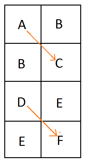
With the ideas of this extension, one way it could look now is this:
The result is that 6 pixels are used instead of 8, for storing the 6 control points of the two quadratic curves.
That isn’t the only result though, so let’s explore the details (:
2. 2D Texture / Quadratic Piecewise Curves
Let’s start by more formally looking at the 2d texture / quadratic curve case.
We are going to number the pixels by their texture coordinate location (in the form of Pyx) instead of using letters. Later on that will help show a pattern of generalization. We are still using the same notation for control points where C0 is the first control point, C1 is the second control point and so on.
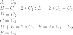
Looking at a single quadratic curve we have this texture which has these constraints on it’s pixel values:
To analyze this, let’s make an augmented matrix. The left matrix is a 3×4 matrix where each column is a pixel and each row is the left side of the equation for a constraint. The right matrix is a 3×3 matrix where each column is a control point and each row is the right side of the equation for a constraint. The first row of the matrix is column labels to help see what’s going on more easily.
Note that i put my pixel columns and control point columns in ascending order in the matrix, but if you put them in a different order, you’d get the same (or equivalent) results as I did. It’s just my convention they are in this order.
![\left[\begin{array}{rrrr|rrr} P_{00} & P_{01} & P_{10} & P_{11} & C_0 & C_1 & C_2 \\ 1 & 0 & 0 & 0 & 1 & 0 & 0 \\ 0 & 1 & 1 & 0 & 0 & 2 & 0\\ 0 & 0 & 0 & 1 & 0 & 0 & 1 \end{array}\right]](https://s0.wp.com/latex.php?latex=%5Cleft%5B%5Cbegin%7Barray%7D%7Brrrr%7Crrr%7D+P_%7B00%7D+%26+P_%7B01%7D+%26+P_%7B10%7D+%26+P_%7B11%7D+%26+C_0+%26+C_1+%26+C_2+%5C%5C+1+%26+0+%26+0+%26+0+%26+1+%26+0+%26+0+%5C%5C+0+%26+1+%26+1+%26+0+%26+0+%26+2+%26+0%5C%5C+0+%26+0+%26+0+%26+1+%26+0+%26+0+%26+1+%5Cend%7Barray%7D%5Cright%5D+&bg=ffffff&fg=666666&s=0&c=20201002)
The next step would be to put this matrix into reduced row echelon form to solve the equations to see what the values of the pixels need to be, but the matrix is in fact already in rref form! (For more information on rref, check out my last post: Solving N equations and N unknowns: The Fine Print (Gauss Jordan Elimination))
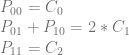
What we can see by looking at the rref of the matrix is that either P01 or P10 can be a free variable – meaning we can choose whatever value we want for it. After we choose a value for either of those variables (pixels), the rest of the pixels are fully defined.
Deciding that P10 is the free variable (just by convention that it isn’t the leading non zero value), the second equation (constraint) becomes P01 = 2*C1-P10.
If we choose the value C1 for P10, that means that P01 must equal C1 too (this is how the original technique worked). If we choose 0 for P10, that means that P01 must equal 2*C1. This is because P01 must always equal 2*C1-P10. We then are in the new territory of this extension, where the pixels representing the middle control point have some freedom about what values they can take on, so long as they average to the middle control point value.
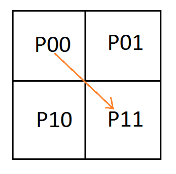
Let’s add a row of pixels and try encoding a second quadratic curve:
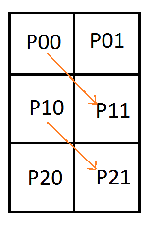
Let’s again make an augmented matrix with pixels on the left and control points on the right.
![\left[\begin{array}{rrrrrr|rrrrrr} P_{00} & P_{01} & P_{10} & P_{11} & P_{20} & P_{21} & C_0 & C_1 & C_2 & C_3 & C_4 & C_5\\ 1 & 0 & 0 & 0 & 0 & 0 & 1 & 0 & 0 & 0 & 0 & 0\\ 0 & 1 & 1 & 0 & 0 & 0 & 0 & 2 & 0 & 0 & 0 & 0 \\ 0 & 0 & 0 & 1 & 0 & 0 & 0 & 0 & 1 & 0 & 0 & 0 \\ 0 & 0 & 1 & 0 & 0 & 0 & 0 & 0 & 0 & 1 & 0 & 0 \\ 0 & 0 & 0 & 1 & 1 & 0 & 0 & 0 & 0 & 0 & 2 & 0 \\ 0 & 0 & 0 & 0 & 0 & 1 & 0 & 0 & 0 & 0 & 0 & 1 \end{array}\right]](https://s0.wp.com/latex.php?latex=%5Cleft%5B%5Cbegin%7Barray%7D%7Brrrrrr%7Crrrrrr%7D+P_%7B00%7D+%26+P_%7B01%7D+%26+P_%7B10%7D+%26+P_%7B11%7D+%26+P_%7B20%7D+%26+P_%7B21%7D+%26+C_0+%26+C_1+%26+C_2+%26+C_3+%26+C_4+%26+C_5%5C%5C+1+%26+0+%26+0+%26+0+%26+0+%26+0+%26+1+%26+0+%26+0+%26+0+%26+0+%26+0%5C%5C+0+%26+1+%26+1+%26+0+%26+0+%26+0+%26+0+%26+2+%26+0+%26+0+%26+0+%26+0+%5C%5C+0+%26+0+%26+0+%26+1+%26+0+%26+0+%26+0+%26+0+%26+1+%26+0+%26+0+%26+0+%5C%5C+0+%26+0+%26+1+%26+0+%26+0+%26+0+%26+0+%26+0+%26+0+%26+1+%26+0+%26+0+%5C%5C+0+%26+0+%26+0+%26+1+%26+1+%26+0+%26+0+%26+0+%26+0+%26+0+%26+2+%26+0+%5C%5C+0+%26+0+%26+0+%26+0+%26+0+%26+1+%26+0+%26+0+%26+0+%26+0+%26+0+%26+1++%5Cend%7Barray%7D%5Cright%5D+&bg=ffffff&fg=666666&s=0&c=20201002)
Putting that into rref to solve for the pixel values we get this:
![\left[\begin{array}{rrrrrr|rrrrrr} P_{00} & P_{01} & P_{10} & P_{11} & P_{20} & P_{21} & C_0 & C_1 & C_2 & C_3 & C_4 & C_5\\ 1 & 0 & 0 & 0 & 0 & 0 & 1 & 0 & 0 & 0 & 0 & 0\\ 0 & 1 & 0 & 0 & 0 & 0 & 0 & 2 & 0 & -1 & 0 & 0 \\ 0 & 0 & 1 & 0 & 0 & 0 & 0 & 0 & 0 & 1 & 0 & 0 \\ 0 & 0 & 0 & 1 & 0 & 0 & 0 & 0 & 1 & 0 & 0 & 0 \\ 0 & 0 & 0 & 0 & 1 & 0 & 0 & 0 & -1 & 0 & 2 & 0 \\ 0 & 0 & 0 & 0 & 0 & 1 & 0 & 0 & 0 & 0 & 0 & 1 \end{array}\right]](https://s0.wp.com/latex.php?latex=%5Cleft%5B%5Cbegin%7Barray%7D%7Brrrrrr%7Crrrrrr%7D+P_%7B00%7D+%26+P_%7B01%7D+%26+P_%7B10%7D+%26+P_%7B11%7D+%26+P_%7B20%7D+%26+P_%7B21%7D+%26+C_0+%26+C_1+%26+C_2+%26+C_3+%26+C_4+%26+C_5%5C%5C+1+%26+0+%26+0+%26+0+%26+0+%26+0+%26+1+%26+0+%26+0+%26+0+%26+0+%26+0%5C%5C+0+%26+1+%26+0+%26+0+%26+0+%26+0+%26+0+%26+2+%26+0+%26+-1+%26+0+%26+0+%5C%5C+0+%26+0+%26+1+%26+0+%26+0+%26+0+%26+0+%26+0+%26+0+%26+1+%26+0+%26+0+%5C%5C+0+%26+0+%26+0+%26+1+%26+0+%26+0+%26+0+%26+0+%26+1+%26+0+%26+0+%26+0+%5C%5C+0+%26+0+%26+0+%26+0+%26+1+%26+0+%26+0+%26+0+%26+-1+%26+0+%26+2+%26+0+%5C%5C+0+%26+0+%26+0+%26+0+%26+0+%26+1+%26+0+%26+0+%26+0+%26+0+%26+0+%26+1++%5Cend%7Barray%7D%5Cright%5D+&bg=ffffff&fg=666666&s=0&c=20201002)
We got the identity matrix on the left, so we don’t have any inconsistencies or free variables.
If we turn that matrix back into equations we get this:

We were successful! We can store two piecewise Bezier curves in 6 pixels by setting the pixel values to these specific values.
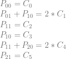
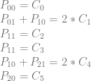
The last example we’ll show is the next stage, where it falls apart. We’ll add another row of pixels and try to encode 3 Bezier curves (9 control points) into those 8 pixels.

This is the augmented matrix with pixels on the left and control points on the right:
![\left[\begin{array}{rrrrrrrr|rrrrrrrrr} P_{00} & P_{01} & P_{10} & P_{11} & P_{20} & P_{21} & P_{30} & P_{31} & C_0 & C_1 & C_2 & C_3 & C_4 & C_5 & C_6 & C_7 & C_8\\ 1 & 0 & 0 & 0 & 0 & 0 & 0 & 0 & 1 & 0 & 0 & 0 & 0 & 0 & 0 & 0 & 0\\ 0 & 1 & 1 & 0 & 0 & 0 & 0 & 0 & 0 & 2 & 0 & 0 & 0 & 0 & 0 & 0 & 0\\ 0 & 0 & 0 & 1 & 0 & 0 & 0 & 0 & 0 & 0 & 1 & 0 & 0 & 0 & 0 & 0 & 0 \\ 0 & 0 & 1 & 0 & 0 & 0 & 0 & 0 & 0 & 0 & 0 & 1 & 0 & 0 & 0 & 0 & 0 \\ 0 & 0 & 0 & 1 & 1 & 0 & 0 & 0 & 0 & 0 & 0 & 0 & 2 & 0 & 0 & 0 & 0 \\ 0 & 0 & 0 & 0 & 0 & 1 & 0 & 0 & 0 & 0 & 0 & 0 & 0 & 1 & 0 & 0 & 0 \\ 0 & 0 & 0 & 0 & 1 & 0 & 0 & 0 & 0 & 0 & 0 & 0 & 0 & 0 & 1 & 0 & 0 \\ 0 & 0 & 0 & 0 & 0 & 1 & 1 & 0 & 0 & 0 & 0 & 0 & 0 & 0 & 0 & 2 & 0 \\ 0 & 0 & 0 & 0 & 0 & 0 & 0 & 1 & 0 & 0 & 0 & 0 & 0 & 0 & 0 & 0 & 1 \\ \end{array}\right]](https://s0.wp.com/latex.php?latex=%5Cleft%5B%5Cbegin%7Barray%7D%7Brrrrrrrr%7Crrrrrrrrr%7D+P_%7B00%7D+%26+P_%7B01%7D+%26+P_%7B10%7D+%26+P_%7B11%7D+%26+P_%7B20%7D+%26+P_%7B21%7D+%26+P_%7B30%7D+%26+P_%7B31%7D+%26+C_0+%26+C_1+%26+C_2+%26+C_3+%26+C_4+%26+C_5+%26+C_6+%26+C_7+%26+C_8%5C%5C+1+%26+0+%26+0+%26+0+%26+0+%26+0+%26+0+%26+0+%26+1+%26+0+%26+0+%26+0+%26+0+%26+0+%26+0+%26+0+%26+0%5C%5C+0+%26+1+%26+1+%26+0+%26+0+%26+0+%26+0+%26+0+%26+0+%26+2+%26+0+%26+0+%26+0+%26+0+%26+0+%26+0+%26+0%5C%5C+0+%26+0+%26+0+%26+1+%26+0+%26+0+%26+0+%26+0+%26+0+%26+0+%26+1+%26+0+%26+0+%26+0+%26+0+%26+0+%26+0+%5C%5C+0+%26+0+%26+1+%26+0+%26+0+%26+0+%26+0+%26+0+%26+0+%26+0+%26+0+%26+1+%26+0+%26+0+%26+0+%26+0+%26+0+%5C%5C+0+%26+0+%26+0+%26+1+%26+1+%26+0+%26+0+%26+0+%26+0+%26+0+%26+0+%26+0+%26+2+%26+0+%26+0+%26+0+%26+0+%5C%5C+0+%26+0+%26+0+%26+0+%26+0+%26+1+%26+0+%26+0+%26+0+%26+0+%26+0+%26+0+%26+0+%26+1+%26+0+%26+0+%26+0+%5C%5C+0+%26+0+%26+0+%26+0+%26+1+%26+0+%26+0+%26+0+%26+0+%26+0+%26+0+%26+0+%26+0+%26+0+%26+1+%26+0+%26+0+%5C%5C+0+%26+0+%26+0+%26+0+%26+0+%26+1+%26+1+%26+0+%26+0+%26+0+%26+0+%26+0+%26+0+%26+0+%26+0+%26+2+%26+0+%5C%5C+0+%26+0+%26+0+%26+0+%26+0+%26+0+%26+0+%26+1+%26+0+%26+0+%26+0+%26+0+%26+0+%26+0+%26+0+%26+0+%26+1+%5C%5C+%5Cend%7Barray%7D%5Cright%5D+&bg=ffffff&fg=666666&s=0&c=20201002)
The rref form is:
![\left[\begin{array}{rrrrrrrr|rrrrrrrrr} P_{00} & P_{01} & P_{10} & P_{11} & P_{20} & P_{21} & P_{30} & P_{31} & C_0 & C_1 & C_2 & C_3 & C_4 & C_5 & C_6 & C_7 & C_8\\ 1 & 0 & 0 & 0 & 0 & 0 & 0 & 0 & 1 & 0 & 0 & 0 & 0 & 0 & 0 & 0 & 0\\ 0 & 1 & 0 & 0 & 0 & 0 & 0 & 0 & 0 & 2 & 0 & -1 & 0 & 0 & 0 & 0 & 0\\ 0 & 0 & 1 & 0 & 0 & 0 & 0 & 0 & 0 & 0 & 0 & 1 & 0 & 0 & 0 & 0 & 0 \\ 0 & 0 & 0 & 1 & 0 & 0 & 0 & 0 & 0 & 0 & 0 & 0 & 2 & 0 & -1 & 0 & 0 \\ 0 & 0 & 0 & 0 & 1 & 0 & 0 & 0 & 0 & 0 & 0 & 0 & 0 & 0 & 1 & 0 & 0 \\ 0 & 0 & 0 & 0 & 0 & 1 & 0 & 0 & 0 & 0 & 0 & 0 & 0 & 1 & 0 & 0 & 0 \\ 0 & 0 & 0 & 0 & 0 & 0 & 1 & 0 & 0 & 0 & 0 & 0 & 0 & -1 & 0 & 2 & 0 \\ 0 & 0 & 0 & 0 & 0 & 0 & 0 & 1 & 0 & 0 & 0 & 0 & 0 & 0 & 0 & 0 & 1 \\ 0 & 0 & 0 & 0 & 0 & 0 & 0 & 0 & 0 & 0 & 1 & 0 & -2 & 0 & 1 & 0 & 0 \\ \end{array}\right]](https://s0.wp.com/latex.php?latex=%5Cleft%5B%5Cbegin%7Barray%7D%7Brrrrrrrr%7Crrrrrrrrr%7D+P_%7B00%7D+%26+P_%7B01%7D+%26+P_%7B10%7D+%26+P_%7B11%7D+%26+P_%7B20%7D+%26+P_%7B21%7D+%26+P_%7B30%7D+%26+P_%7B31%7D+%26+C_0+%26+C_1+%26+C_2+%26+C_3+%26+C_4+%26+C_5+%26+C_6+%26+C_7+%26+C_8%5C%5C+1+%26+0+%26+0+%26+0+%26+0+%26+0+%26+0+%26+0+%26+1+%26+0+%26+0+%26+0+%26+0+%26+0+%26+0+%26+0+%26+0%5C%5C+0+%26+1+%26+0+%26+0+%26+0+%26+0+%26+0+%26+0+%26+0+%26+2+%26+0+%26+-1+%26+0+%26+0+%26+0+%26+0+%26+0%5C%5C+0+%26+0+%26+1+%26+0+%26+0+%26+0+%26+0+%26+0+%26+0+%26+0+%26+0+%26+1+%26+0+%26+0+%26+0+%26+0+%26+0+%5C%5C+0+%26+0+%26+0+%26+1+%26+0+%26+0+%26+0+%26+0+%26+0+%26+0+%26+0+%26+0+%26+2+%26+0+%26+-1+%26+0+%26+0+%5C%5C+0+%26+0+%26+0+%26+0+%26+1+%26+0+%26+0+%26+0+%26+0+%26+0+%26+0+%26+0+%26+0+%26+0+%26+1+%26+0+%26+0+%5C%5C+0+%26+0+%26+0+%26+0+%26+0+%26+1+%26+0+%26+0+%26+0+%26+0+%26+0+%26+0+%26+0+%26+1+%26+0+%26+0+%26+0+%5C%5C+0+%26+0+%26+0+%26+0+%26+0+%26+0+%26+1+%26+0+%26+0+%26+0+%26+0+%26+0+%26+0+%26+-1+%26+0+%26+2+%26+0+%5C%5C+0+%26+0+%26+0+%26+0+%26+0+%26+0+%26+0+%26+1+%26+0+%26+0+%26+0+%26+0+%26+0+%26+0+%26+0+%26+0+%26+1+%5C%5C+0+%26+0+%26+0+%26+0+%26+0+%26+0+%26+0+%26+0+%26+0+%26+0+%26+1+%26+0+%26+-2+%26+0+%26+1+%26+0+%26+0+%5C%5C+%5Cend%7Barray%7D%5Cright%5D+&bg=ffffff&fg=666666&s=0&c=20201002)
Let’s turn that back into equations.
We have a problem unfortunately! The bottom row says this:

That means that we can only store these curves in this pixel configuration if we limit the values of the control points 2,4,6 to values that make that last equation true.
Since my desire is to be able to store curves in textures without “unusual” restrictions on what the control points can be, I’m going to count this as a failure for a general case solution.
It only gets worse from here for the case of trying to add another row of pixels for each curve you want to add.
It looks like storing two quadratic curves in a 2×6 group of pixels is the most optimal (data dense) storage. If you go any higher, it puts restrictions on the control points. If you go any lower, you have a free variable, which means you aren’t making full use of all of the pixels you have.
This means that if you are storing piecewise quadratic curves in 2d textures, doing it this way will cause you to use 3/4 as many pixels as doing it the other way, and you will be using 1 pixel per control point stored, instead of 1.333 pixels per control point stored.
This isn’t the end of the story though, so let’s continue (:
3. 2D Texture / Quadratic Piecewise Curves – C0 Continuity
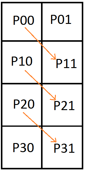
If we add the requirement that our piecewise curves must be connected (aka that they have C0 continuity), we can actually do something pretty interesting. Take a look at this setup:
Putting this into matrix form looks like this:
![\left[\begin{array}{rrrrrr|rrrrrr} P_{00} & P_{01} & P_{10} & P_{11} & P_{20} & P_{21} & C_0 & C_1 & C_2 & C_3 & C_4 & C_5\\ 1 & 0 & 0 & 0 & 0 & 0 & 1 & 0 & 0 & 0 & 0 & 0\\ 0 & 1 & 1 & 0 & 0 & 0 & 0 & 2 & 0 & 0 & 0 & 0 \\ 0 & 0 & 0 & 1 & 0 & 0 & 0 & 0 & 1 & 0 & 0 & 0 \\ 0 & 0 & 0 & 1 & 0 & 0 & 0 & 0 & 0 & 1 & 0 & 0 \\ 0 & 0 & 1 & 0 & 0 & 1 & 0 & 0 & 0 & 0 & 2 & 0 \\ 0 & 0 & 0 & 0 & 1 & 0 & 0 & 0 & 0 & 0 & 0 & 1 \\ \end{array}\right]](https://s0.wp.com/latex.php?latex=%5Cleft%5B%5Cbegin%7Barray%7D%7Brrrrrr%7Crrrrrr%7D+P_%7B00%7D+%26+P_%7B01%7D+%26+P_%7B10%7D+%26+P_%7B11%7D+%26+P_%7B20%7D+%26+P_%7B21%7D+%26+C_0+%26+C_1+%26+C_2+%26+C_3+%26+C_4+%26+C_5%5C%5C+1+%26+0+%26+0+%26+0+%26+0+%26+0+%26+1+%26+0+%26+0+%26+0+%26+0+%26+0%5C%5C+0+%26+1+%26+1+%26+0+%26+0+%26+0+%26+0+%26+2+%26+0+%26+0+%26+0+%26+0+%5C%5C+0+%26+0+%26+0+%26+1+%26+0+%26+0+%26+0+%26+0+%26+1+%26+0+%26+0+%26+0+%5C%5C+0+%26+0+%26+0+%26+1+%26+0+%26+0+%26+0+%26+0+%26+0+%26+1+%26+0+%26+0+%5C%5C+0+%26+0+%26+1+%26+0+%26+0+%26+1+%26+0+%26+0+%26+0+%26+0+%26+2+%26+0+%5C%5C+0+%26+0+%26+0+%26+0+%26+1+%26+0+%26+0+%26+0+%26+0+%26+0+%26+0+%26+1+%5C%5C+%5Cend%7Barray%7D%5Cright%5D+&bg=ffffff&fg=666666&s=0&c=20201002)
In rref it becomes this:
![\left[\begin{array}{rrrrrr|rrrrrr} P_{00} & P_{01} & P_{10} & P_{11} & P_{20} & P_{21} & C_0 & C_1 & C_2 & C_3 & C_4 & C_5\\ 1 & 0 & 0 & 0 & 0 & 0 & 1 & 0 & 0 & 0 & 0 & 0\\ 0 & 1 & 0 & 0 & 0 & -1 & 0 & 2 & 0 & 0 & -2 & 0 \\ 0 & 0 & 1 & 0 & 0 & 1 & 0 & 0 & 0 & 0 & 2 & 0 \\ 0 & 0 & 0 & 1 & 0 & 0 & 0 & 0 & 0 & 1 & 0 & 0 \\ 0 & 0 & 0 & 0 & 1 & 0 & 0 & 0 & 0 & 0 & 0 & 1 \\ 0 & 0 & 0 & 0 & 0 & 0 & 0 & 0 & 1 & -1 & 0 & 0 \\ \end{array}\right]](https://s0.wp.com/latex.php?latex=%5Cleft%5B%5Cbegin%7Barray%7D%7Brrrrrr%7Crrrrrr%7D+P_%7B00%7D+%26+P_%7B01%7D+%26+P_%7B10%7D+%26+P_%7B11%7D+%26+P_%7B20%7D+%26+P_%7B21%7D+%26+C_0+%26+C_1+%26+C_2+%26+C_3+%26+C_4+%26+C_5%5C%5C+1+%26+0+%26+0+%26+0+%26+0+%26+0+%26+1+%26+0+%26+0+%26+0+%26+0+%26+0%5C%5C+0+%26+1+%26+0+%26+0+%26+0+%26+-1+%26+0+%26+2+%26+0+%26+0+%26+-2+%26+0+%5C%5C+0+%26+0+%26+1+%26+0+%26+0+%26+1+%26+0+%26+0+%26+0+%26+0+%26+2+%26+0+%5C%5C+0+%26+0+%26+0+%26+1+%26+0+%26+0+%26+0+%26+0+%26+0+%26+1+%26+0+%26+0+%5C%5C+0+%26+0+%26+0+%26+0+%26+1+%26+0+%26+0+%26+0+%26+0+%26+0+%26+0+%26+1+%5C%5C+0+%26+0+%26+0+%26+0+%26+0+%26+0+%26+0+%26+0+%26+1+%26+-1+%26+0+%26+0+%5C%5C+%5Cend%7Barray%7D%5Cright%5D+&bg=ffffff&fg=666666&s=0&c=20201002)
Turning the rref back into equations we get:

P21 is a free variable, so we can set it to whatever we want. Once we choose a value, the pixel values P01 and P10 will be fully defined.
The bottom equation might have you worried, because it looks like an inconsistency (aka restriction) but it is actually expected.
That last equation says 0 = C2-C3 which can be rearranged into C2 = C3. That just means that the end of our first curve has to equal the beginning of our second curve. That is C0 just the continuity we already said we’d agree to.
So, it worked! Let’s try adding a row of pixels and another curve to see what happens.

Putting that into matrix form:
![\left[\begin{array}{rrrrrrrr|rrrrrrrrr} P_{00} & P_{01} & P_{10} & P_{11} & P_{20} & P_{21} & P_{30} & P_{31} & C_0 & C_1 & C_2 & C_3 & C_4 & C_5 & C_6 & C_7 & C_8\\ 1 & 0 & 0 & 0 & 0 & 0 & 0 & 0 & 1 & 0 & 0 & 0 & 0 & 0 & 0 & 0 & 0\\ 0 & 1 & 1 & 0 & 0 & 0 & 0 & 0 & 0 & 2 & 0 & 0 & 0 & 0 & 0 & 0 & 0\\ 0 & 0 & 0 & 1 & 0 & 0 & 0 & 0 & 0 & 0 & 1 & 0 & 0 & 0 & 0 & 0 & 0\\ 0 & 0 & 0 & 1 & 0 & 0 & 0 & 0 & 0 & 0 & 0 & 1 & 0 & 0 & 0 & 0 & 0\\ 0 & 0 & 1 & 0 & 0 & 1 & 0 & 0 & 0 & 0 & 0 & 0 & 2 & 0 & 0 & 0 & 0\\ 0 & 0 & 0 & 0 & 1 & 0 & 0 & 0 & 0 & 0 & 0 & 0 & 0 & 1 & 0 & 0 & 0\\ 0 & 0 & 0 & 0 & 1 & 0 & 0 & 0 & 0 & 0 & 0 & 0 & 0 & 0 & 1 & 0 & 0\\ 0 & 0 & 0 & 0 & 0 & 1 & 1 & 0 & 0 & 0 & 0 & 0 & 0 & 0 & 0 & 2 & 0\\ 0 & 0 & 0 & 0 & 0 & 0 & 0 & 1 & 0 & 0 & 0 & 0 & 0 & 0 & 0 & 0 & 1\\ \end{array}\right]](https://s0.wp.com/latex.php?latex=%5Cleft%5B%5Cbegin%7Barray%7D%7Brrrrrrrr%7Crrrrrrrrr%7D+P_%7B00%7D+%26+P_%7B01%7D+%26+P_%7B10%7D+%26+P_%7B11%7D+%26+P_%7B20%7D+%26+P_%7B21%7D+%26+P_%7B30%7D+%26+P_%7B31%7D+%26+C_0+%26+C_1+%26+C_2+%26+C_3+%26+C_4+%26+C_5+%26+C_6+%26+C_7+%26+C_8%5C%5C+1+%26+0+%26+0+%26+0+%26+0+%26+0+%26+0+%26+0+%26+1+%26+0+%26+0+%26+0+%26+0+%26+0+%26+0+%26+0+%26+0%5C%5C+0+%26+1+%26+1+%26+0+%26+0+%26+0+%26+0+%26+0+%26+0+%26+2+%26+0+%26+0+%26+0+%26+0+%26+0+%26+0+%26+0%5C%5C+0+%26+0+%26+0+%26+1+%26+0+%26+0+%26+0+%26+0+%26+0+%26+0+%26+1+%26+0+%26+0+%26+0+%26+0+%26+0+%26+0%5C%5C+0+%26+0+%26+0+%26+1+%26+0+%26+0+%26+0+%26+0+%26+0+%26+0+%26+0+%26+1+%26+0+%26+0+%26+0+%26+0+%26+0%5C%5C+0+%26+0+%26+1+%26+0+%26+0+%26+1+%26+0+%26+0+%26+0+%26+0+%26+0+%26+0+%26+2+%26+0+%26+0+%26+0+%26+0%5C%5C+0+%26+0+%26+0+%26+0+%26+1+%26+0+%26+0+%26+0+%26+0+%26+0+%26+0+%26+0+%26+0+%26+1+%26+0+%26+0+%26+0%5C%5C+0+%26+0+%26+0+%26+0+%26+1+%26+0+%26+0+%26+0+%26+0+%26+0+%26+0+%26+0+%26+0+%26+0+%26+1+%26+0+%26+0%5C%5C+0+%26+0+%26+0+%26+0+%26+0+%26+1+%26+1+%26+0+%26+0+%26+0+%26+0+%26+0+%26+0+%26+0+%26+0+%26+2+%26+0%5C%5C+0+%26+0+%26+0+%26+0+%26+0+%26+0+%26+0+%26+1+%26+0+%26+0+%26+0+%26+0+%26+0+%26+0+%26+0+%26+0+%26+1%5C%5C+%5Cend%7Barray%7D%5Cright%5D+&bg=ffffff&fg=666666&s=0&c=20201002)
And in rref:
![\left[\begin{array}{rrrrrrrr|rrrrrrrrr} P_{00} & P_{01} & P_{10} & P_{11} & P_{20} & P_{21} & P_{30} & P_{31} & C_0 & C_1 & C_2 & C_3 & C_4 & C_5 & C_6 & C_7 & C_8\\ 1 & 0 & 0 & 0 & 0 & 0 & 0 & 0 & 1 & 0 & 0 & 0 & 0 & 0 & 0 & 0 & 0\\ 0 & 1 & 0 & 0 & 0 & 0 & 1 & 0 & 0 & 2 & 0 & 0 & -2 & 0 & 0 & 2 & 0\\ 0 & 0 & 1 & 0 & 0 & 0 & -1 & 0 & 0 & 0 & 0 & 0 & 2 & 0 & 0 & -2 & 0\\ 0 & 0 & 0 & 1 & 0 & 0 & 0 & 0 & 0 & 0 & 0 & 1 & 0 & 0 & 0 & 0 & 0\\ 0 & 0 & 0 & 0 & 1 & 0 & 0 & 0 & 0 & 0 & 0 & 0 & 0 & 0 & 1 & 0 & 0\\ 0 & 0 & 0 & 0 & 0 & 1 & 1 & 0 & 0 & 0 & 0 & 0 & 0 & 0 & 0 & 2 & 0\\ 0 & 0 & 0 & 0 & 0 & 0 & 0 & 1 & 0 & 0 & 0 & 0 & 0 & 0 & 0 & 0 & 1\\ 0 & 0 & 0 & 0 & 0 & 0 & 0 & 0 & 0 & 0 & 1 & -1 & 0 & 0 & 0 & 0 & 0\\ 0 & 0 & 0 & 0 & 0 & 0 & 0 & 0 & 0 & 0 & 0 & 0 & 0 & 1 & -1 & 0 & 0\\ \end{array}\right]](https://s0.wp.com/latex.php?latex=%5Cleft%5B%5Cbegin%7Barray%7D%7Brrrrrrrr%7Crrrrrrrrr%7D+P_%7B00%7D+%26+P_%7B01%7D+%26+P_%7B10%7D+%26+P_%7B11%7D+%26+P_%7B20%7D+%26+P_%7B21%7D+%26+P_%7B30%7D+%26+P_%7B31%7D+%26+C_0+%26+C_1+%26+C_2+%26+C_3+%26+C_4+%26+C_5+%26+C_6+%26+C_7+%26+C_8%5C%5C+1+%26+0+%26+0+%26+0+%26+0+%26+0+%26+0+%26+0+%26+1+%26+0+%26+0+%26+0+%26+0+%26+0+%26+0+%26+0+%26+0%5C%5C+0+%26+1+%26+0+%26+0+%26+0+%26+0+%26+1+%26+0+%26+0+%26+2+%26+0+%26+0+%26+-2+%26+0+%26+0+%26+2+%26+0%5C%5C+0+%26+0+%26+1+%26+0+%26+0+%26+0+%26+-1+%26+0+%26+0+%26+0+%26+0+%26+0+%26+2+%26+0+%26+0+%26+-2+%26+0%5C%5C+0+%26+0+%26+0+%26+1+%26+0+%26+0+%26+0+%26+0+%26+0+%26+0+%26+0+%26+1+%26+0+%26+0+%26+0+%26+0+%26+0%5C%5C+0+%26+0+%26+0+%26+0+%26+1+%26+0+%26+0+%26+0+%26+0+%26+0+%26+0+%26+0+%26+0+%26+0+%26+1+%26+0+%26+0%5C%5C+0+%26+0+%26+0+%26+0+%26+0+%26+1+%26+1+%26+0+%26+0+%26+0+%26+0+%26+0+%26+0+%26+0+%26+0+%26+2+%26+0%5C%5C+0+%26+0+%26+0+%26+0+%26+0+%26+0+%26+0+%26+1+%26+0+%26+0+%26+0+%26+0+%26+0+%26+0+%26+0+%26+0+%26+1%5C%5C+0+%26+0+%26+0+%26+0+%26+0+%26+0+%26+0+%26+0+%26+0+%26+0+%26+1+%26+-1+%26+0+%26+0+%26+0+%26+0+%26+0%5C%5C+0+%26+0+%26+0+%26+0+%26+0+%26+0+%26+0+%26+0+%26+0+%26+0+%26+0+%26+0+%26+0+%26+1+%26+-1+%26+0+%26+0%5C%5C+%5Cend%7Barray%7D%5Cright%5D+&bg=ffffff&fg=666666&s=0&c=20201002)
Turning the rref back into equations:

We see that P30 is a free variable, and the last two rows show us we have the C0 continuity requirements: C2 = C3 and C5 = C6.
The last section without C0 continuity reached it’s limit of storage space efficiency after storing two curves (6 control points) in 6 pixels.
When we add the C0 continuity requirement, we were able to take it further and store 3 curves in 8 pixels. Technically those 3 curves have 9 control points, but because the end point of each curve has to be the same as the start point of the next curve it makes it so in reality there is only 3 control points for the first curve and then 2 additional control points for each additional curve. That makes 8 control points for 3 curves, not 9.
Unlike the last section, using this zigzag pattern with C0 continuity, you can encode any number of curves. I am not sure how to prove it, but from observation, there is no sign of any shrinking of capacity as we increase the number of curves, adding two more rows of pixels for each curve. If you know how to prove this more formally, please let me know!
Note that instead of explicitly having 3 control points per curve, where the first control point of a curve has to equal the last control point of the previous curve, you can instead describe the piecewise curves with fewer control points. You need 3 control points for the first curve, and then 2 control points for each curve after that.
Mathematically both ways are equivelant and you’ll get to the same answer. The accompanying source code works that way, but I show this example in this longer way to more explicitly show how things work.
4. 2D Texture / Quadratic Piecewise Curves – Storage Efficiency
Let’s compare the storage efficiency of the last two sections to each other, as well as to the original technique.


The tables show that the first method uses fewer pixels per control point, while the second method uses fewer pixels per curve.
The first method can get you to what I believe to be the maximum density of 1 pixel per control point if you store an even number of curves. It can also give you a curve for every 3 pixels of storage.
The second method approaches the 1 pixel per control point as you store more and more curves and also approaches 2 pixels of storage per curve stored. Note that the second method’s table is using the convention of 3 control points are used for the first curve, and 2 additional control points for each curve after that.
The deciding factor for which method to use is probably going to be whether or not you want to force C0 continuity of your curve data. If so, you’d use the second technique, else you’d use the first.
The original technique uses a constant 1.33 pixels per control point, and 4 pixels to store each curve. Those numbers shows how this extension improves on the storage efficiency of the original technique.
5. Real World Limitations
This extension has a problem that the original technique does not have unfortunately.
While the stuff above is correct mathematically, there are limitations on the values we can store in actual textures. For instance, if we have 8 bit uint8 color channels we can only store values 0 to 255.
Looking at one of the equations  , if C1 is 255 and C3 is 0, we are going to need to store 510 in the 8 bits we have for P01, which we can’t. If C1 is 0 and C3 is not zero, we are going to have to store a negative value in the 8 bits we have for P01, which we can’t.
This becomes less of a problem when using 16 bit floats per color channel, and is basically solved when using 32 bit floats per color channels, but that makes the technique hungrier for storage and less efficient again.
While that limits the usefulness of this extension, there are situations where this would still be appropriate – like if you already have your data stored in 16 or 32 bit color channels like some data (eg position data) would require..
The extension goes further, into 3d textures and beyond though, so let’s explore a little bit more.
6. 3D Texture / Cubic Piecewise Curves
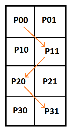
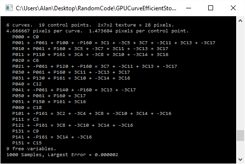
The original technique talks about how to use a 2x2x2 3d volume texture to store a cubic Bezier curve (per color channel) and to retrieve it by doing a trilinear interpolated texture read.
If you have four control points A,B,C,D then the first slice of the volume texture will be a 2d texture storing the quadratic Bezier curve defined by A,B,C and the second slice will store B,C,D. You still sample along the diagonal of the texture but this time it’s a 3d diagonal instead of 2d. Here is that setup, where the texture is sampled along the diagonal from from A to D:

Let’s look at what this extension means for 3d textures / cubic curves.
The equation for a cubic Bezier curve looks like this:

If we derive that from trilinear interpolation between 8 points A,B,C,D,E,F,G,H, the second to last step would look like this:

So, similar to our 2d setup, we have some freedom about our values.
In the original technique, B,C,E would have to be equal to the second control point, and D,F,G would have to be equal to the third control point. With the new extension, in both cases, those groups of values only have to AVERAGE to their specific control points. Once again, this gives us some freedoms for the values we can use, and lets us use our pixels more efficiently.
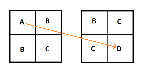
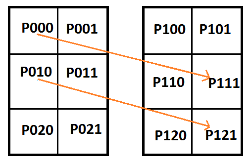
Here is the setup, again using texture coordinates (in the form Pzyx) for the pixels instead of letters.

here’s how the equations look in matrix form, which also happens to already be in rref:
![\left[\begin{array}{rrrrrrrr|rrrr} P_{000} & P_{001} & P_{010} & P_{011} & P_{100} & P_{101} & P_{110} & P_{111} & C_0 & C_1 & C_2 & C_3 \\ 1 & 0 & 0 & 0 & 0 & 0 & 0 & 0 & 1 & 0 & 0 & 0 \\ 0 & 1 & 1 & 0 & 1 & 0 & 0 & 0 & 0 & 3 & 0 & 0 \\ 0 & 0 & 0 & 1 & 0 & 1 & 1 & 0 & 0 & 0 & 3 & 0 \\ 0 & 0 & 0 & 0 & 0 & 0 & 0 & 1 & 0 & 0 & 0 & 1 \\ \end{array}\right]](https://s0.wp.com/latex.php?latex=%5Cleft%5B%5Cbegin%7Barray%7D%7Brrrrrrrr%7Crrrr%7D+P_%7B000%7D+%26+P_%7B001%7D+%26+P_%7B010%7D+%26+P_%7B011%7D+%26+P_%7B100%7D+%26+P_%7B101%7D+%26+P_%7B110%7D+%26+P_%7B111%7D+%26++++C_0+%26+C_1+%26+C_2+%26+C_3+%5C%5C+1+%26+0+%26+0+%26+0+%26+0+%26+0+%26+0+%26+0+%26++++1+%26+0+%26+0+%26+0+%5C%5C+0+%26+1+%26+1+%26+0+%26+1+%26+0+%26+0+%26+0+%26++++0+%26+3+%26+0+%26+0+%5C%5C+0+%26+0+%26+0+%26+1+%26+0+%26+1+%26+1+%26+0+%26++++0+%26+0+%26+3+%26+0+%5C%5C+0+%26+0+%26+0+%26+0+%26+0+%26+0+%26+0+%26+1+%26++++0+%26+0+%26+0+%26+1+%5C%5C+%5Cend%7Barray%7D%5Cright%5D+&bg=ffffff&fg=666666&s=0&c=20201002)
P010 and P100 are free variables and so are P101 and P110, making a total of four free variables. They can be set to any value desired, which will then define the value that P001 and P011 need to be.
Let’s add another piecewise cubic Bezier curve, and another row of pixels to the texture to see what happens.

Here are the equations in matrix form:
![\left[\begin{array}{rrrrrrrrrrrr|rrrrrrrr} P_{000} & P_{001} & P_{010} & P_{011} & P_{020} & P_{021} & P_{100} & P_{101} & P_{110} & P_{111} & P_{120} & P_{121} & C_{0} & C_{1} & C_{2} & C_{3} & C_{4} & C_{5} & C_{6} & C_{7} \\ 1 & 0 & 0 & 0 & 0 & 0 & 0 & 0 & 0 & 0 & 0 & 0 & 1 & 0 & 0 & 0 & 0 & 0 & 0 & 0 \\ 0 & 1 & 1 & 0 & 0 & 0 & 1 & 0 & 0 & 0 & 0 & 0 & 0 & 3 & 0 & 0 & 0 & 0 & 0 & 0 \\ 0 & 0 & 0 & 1 & 0 & 0 & 0 & 1 & 1 & 0 & 0 & 0 & 0 & 0 & 3 & 0 & 0 & 0 & 0 & 0 \\ 0 & 0 & 0 & 0 & 0 & 0 & 0 & 0 & 0 & 1 & 0 & 0 & 0 & 0 & 0 & 1 & 0 & 0 & 0 & 0 \\ 0 & 0 & 1 & 0 & 0 & 0 & 0 & 0 & 0 & 0 & 0 & 0 & 0 & 0 & 0 & 0 & 1 & 0 & 0 & 0 \\ 0 & 0 & 0 & 1 & 1 & 0 & 0 & 0 & 1 & 0 & 0 & 0 & 0 & 0 & 0 & 0 & 0 & 3 & 0 & 0 \\ 0 & 0 & 0 & 0 & 0 & 1 & 0 & 0 & 0 & 1 & 1 & 0 & 0 & 0 & 0 & 0 & 0 & 0 & 3 & 0 \\ 0 & 0 & 0 & 0 & 0 & 0 & 0 & 0 & 0 & 0 & 0 & 1 & 0 & 0 & 0 & 0 & 0 & 0 & 0 & 1 \\ \end{array}\right]](https://s0.wp.com/latex.php?latex=%5Cleft%5B%5Cbegin%7Barray%7D%7Brrrrrrrrrrrr%7Crrrrrrrr%7D+P_%7B000%7D+%26+P_%7B001%7D+%26+P_%7B010%7D+%26+P_%7B011%7D+%26+P_%7B020%7D+%26+P_%7B021%7D+%26+P_%7B100%7D+%26+P_%7B101%7D+%26+P_%7B110%7D+%26+P_%7B111%7D+%26+P_%7B120%7D+%26+P_%7B121%7D+%26+C_%7B0%7D+%26+C_%7B1%7D+%26+C_%7B2%7D+%26+C_%7B3%7D+%26+C_%7B4%7D+%26+C_%7B5%7D+%26+C_%7B6%7D+%26+C_%7B7%7D+%5C%5C+1+%26+0+%26+0+%26+0+%26+0+%26+0+%26+0+%26+0+%26+0+%26+0+%26+0+%26+0+%26+1+%26+0+%26+0+%26+0+%26+0+%26+0+%26+0+%26+0+%5C%5C+0+%26+1+%26+1+%26+0+%26+0+%26+0+%26+1+%26+0+%26+0+%26+0+%26+0+%26+0+%26+0+%26+3+%26+0+%26+0+%26+0+%26+0+%26+0+%26+0+%5C%5C+0+%26+0+%26+0+%26+1+%26+0+%26+0+%26+0+%26+1+%26+1+%26+0+%26+0+%26+0+%26+0+%26+0+%26+3+%26+0+%26+0+%26+0+%26+0+%26+0+%5C%5C+0+%26+0+%26+0+%26+0+%26+0+%26+0+%26+0+%26+0+%26+0+%26+1+%26+0+%26+0+%26+0+%26+0+%26+0+%26+1+%26+0+%26+0+%26+0+%26+0+%5C%5C+0+%26+0+%26+1+%26+0+%26+0+%26+0+%26+0+%26+0+%26+0+%26+0+%26+0+%26+0+%26+0+%26+0+%26+0+%26+0+%26+1+%26+0+%26+0+%26+0+%5C%5C+0+%26+0+%26+0+%26+1+%26+1+%26+0+%26+0+%26+0+%26+1+%26+0+%26+0+%26+0+%26+0+%26+0+%26+0+%26+0+%26+0+%26+3+%26+0+%26+0+%5C%5C+0+%26+0+%26+0+%26+0+%26+0+%26+1+%26+0+%26+0+%26+0+%26+1+%26+1+%26+0+%26+0+%26+0+%26+0+%26+0+%26+0+%26+0+%26+3+%26+0+%5C%5C+0+%26+0+%26+0+%26+0+%26+0+%26+0+%26+0+%26+0+%26+0+%26+0+%26+0+%26+1+%26+0+%26+0+%26+0+%26+0+%26+0+%26+0+%26+0+%26+1+%5C%5C+%5Cend%7Barray%7D%5Cright%5D+&bg=ffffff&fg=666666&s=0&c=20201002)
Here it is in rref:
![\left[\begin{array}{rrrrrrrrrrrr|rrrrrrrr} P_{000} & P_{001} & P_{010} & P_{011} & P_{020} & P_{021} & P_{100} & P_{101} & P_{110} & P_{111} & P_{120} & P_{121} & C_{0} & C_{1} & C_{2} & C_{3} & C_{4} & C_{5} & C_{6} & C_{7} \\ 1 & 0 & 0 & 0 & 0 & 0 & 0 & 0 & 0 & 0 & 0 & 0 & 1 & 0 & 0 & 0 & 0 & 0 & 0 & 0 \\ 0 & 1 & 0 & 0 & 0 & 0 & 1 & 0 & 0 & 0 & 0 & 0 & 0 & 3 & 0 & 0 & -1 & 0 & 0 & 0 \\ 0 & 0 & 1 & 0 & 0 & 0 & 0 & 0 & 0 & 0 & 0 & 0 & 0 & 0 & 0 & 0 & 1 & 0 & 0 & 0 \\ 0 & 0 & 0 & 1 & 0 & 0 & 0 & 1 & 1 & 0 & 0 & 0 & 0 & 0 & 3 & 0 & 0 & 0 & 0 & 0 \\ 0 & 0 & 0 & 0 & 1 & 0 & 0 & -1 & 0 & 0 & 0 & 0 & 0 & 0 & -3 & 0 & 0 & 3 & 0 & 0 \\ 0 & 0 & 0 & 0 & 0 & 1 & 0 & 0 & 0 & 0 & 1 & 0 & 0 & 0 & 0 & -1 & 0 & 0 & 3 & 0 \\ 0 & 0 & 0 & 0 & 0 & 0 & 0 & 0 & 0 & 1 & 0 & 0 & 0 & 0 & 0 & 1 & 0 & 0 & 0 & 0 \\ 0 & 0 & 0 & 0 & 0 & 0 & 0 & 0 & 0 & 0 & 0 & 1 & 0 & 0 & 0 & 0 & 0 & 0 & 0 & 1 \\ \end{array}\right]](https://s0.wp.com/latex.php?latex=%5Cleft%5B%5Cbegin%7Barray%7D%7Brrrrrrrrrrrr%7Crrrrrrrr%7D+P_%7B000%7D+%26+P_%7B001%7D+%26+P_%7B010%7D+%26+P_%7B011%7D+%26+P_%7B020%7D+%26+P_%7B021%7D+%26+P_%7B100%7D+%26+P_%7B101%7D+%26+P_%7B110%7D+%26+P_%7B111%7D+%26+P_%7B120%7D+%26+P_%7B121%7D+%26+C_%7B0%7D+%26+C_%7B1%7D+%26+C_%7B2%7D+%26+C_%7B3%7D+%26+C_%7B4%7D+%26+C_%7B5%7D+%26+C_%7B6%7D+%26+C_%7B7%7D+%5C%5C+1+%26+0+%26+0+%26+0+%26+0+%26+0+%26+0+%26+0+%26+0+%26+0+%26+0+%26+0+%26+1+%26+0+%26+0+%26+0+%26+0+%26+0+%26+0+%26+0+%5C%5C+0+%26+1+%26+0+%26+0+%26+0+%26+0+%26+1+%26+0+%26+0+%26+0+%26+0+%26+0+%26+0+%26+3+%26+0+%26+0+%26+-1+%26+0+%26+0+%26+0+%5C%5C+0+%26+0+%26+1+%26+0+%26+0+%26+0+%26+0+%26+0+%26+0+%26+0+%26+0+%26+0+%26+0+%26+0+%26+0+%26+0+%26+1+%26+0+%26+0+%26+0+%5C%5C+0+%26+0+%26+0+%26+1+%26+0+%26+0+%26+0+%26+1+%26+1+%26+0+%26+0+%26+0+%26+0+%26+0+%26+3+%26+0+%26+0+%26+0+%26+0+%26+0+%5C%5C+0+%26+0+%26+0+%26+0+%26+1+%26+0+%26+0+%26+-1+%26+0+%26+0+%26+0+%26+0+%26+0+%26+0+%26+-3+%26+0+%26+0+%26+3+%26+0+%26+0+%5C%5C+0+%26+0+%26+0+%26+0+%26+0+%26+1+%26+0+%26+0+%26+0+%26+0+%26+1+%26+0+%26+0+%26+0+%26+0+%26+-1+%26+0+%26+0+%26+3+%26+0+%5C%5C+0+%26+0+%26+0+%26+0+%26+0+%26+0+%26+0+%26+0+%26+0+%26+1+%26+0+%26+0+%26+0+%26+0+%26+0+%26+1+%26+0+%26+0+%26+0+%26+0+%5C%5C+0+%26+0+%26+0+%26+0+%26+0+%26+0+%26+0+%26+0+%26+0+%26+0+%26+0+%26+1+%26+0+%26+0+%26+0+%26+0+%26+0+%26+0+%26+0+%26+1+%5C%5C+%5Cend%7Barray%7D%5Cright%5D+&bg=ffffff&fg=666666&s=0&c=20201002)
Putting that back into equations we have this:

The result is that we still have four free variables: P100, P101, P110 and P120. When we give values to those pixels, we will then be able to calculate the values for P001, P011, P020 and P021.
There is a limit to this pattern though. Where the maximum number of curves to follow the pattern was 2 with the 2d / quadratic case, the maximum number of curves to follow this pattern with the 3d / cubic case is 3. As soon as you try to put 4 curves in this pattern it fails by having constraints. Interestingly, we still have 4 free variables when putting 3 curves in there, so it doesn’t follow the 2d case where free variables disappeared as we put more curves in, indicating when the failure would happen.
If you know how to more formally analyze when these patterns of equations will fail, please let me know!
7. 3D Texture / Cubic Piecewise Curves – Multiple Curves?
Looking at the 3d texture case of 2x2x2 storing a single curve, I saw that there were 4 free variables. Since it takes 4 control points to define a cubic curve, I wondered if we could use those 4 free variables to encode another cubic curve.
Here’s a setup where the x axis is flipped for the second curve. It’s a little bit hard to tell from the diagram, but the blue line does still go through the center of the 3d cube. It goes from P001 to P110, while the first curve still goes from P000 to P111.

Here’s what the equations look like:

And in matrix form:
![\left[\begin{array}{rrrrrrrr|rrrrrrrr} P_{000} & P_{001} & P_{010} & P_{011} & P_{100} & P_{101} & P_{110} & P_{111} & C_{0} & C_{1} & C_{2} & C_{3} & C_{4} & C_{5} & C_{6} & C_{7} \\ 1 & 0 & 0 & 0 & 0 & 0 & 0 & 0 & 1 & 0 & 0 & 0 & 0 & 0 & 0 & 0 \\ 0 & 1 & 1 & 0 & 1 & 0 & 0 & 0 & 0 & 3 & 0 & 0 & 0 & 0 & 0 & 0 \\ 0 & 0 & 0 & 1 & 0 & 1 & 1 & 0 & 0 & 0 & 3 & 0 & 0 & 0 & 0 & 0 \\ 0 & 0 & 0 & 0 & 0 & 0 & 0 & 1 & 0 & 0 & 0 & 1 & 0 & 0 & 0 & 0 \\ 0 & 1 & 0 & 0 & 0 & 0 & 0 & 0 & 0 & 0 & 0 & 0 & 1 & 0 & 0 & 0 \\ 1 & 0 & 0 & 1 & 0 & 1 & 0 & 0 & 0 & 0 & 0 & 0 & 0 & 3 & 0 & 0 \\ 0 & 0 & 1 & 0 & 1 & 0 & 0 & 1 & 0 & 0 & 0 & 0 & 0 & 0 & 3 & 0 \\ 0 & 0 & 0 & 0 & 0 & 0 & 1 & 0 & 0 & 0 & 0 & 0 & 0 & 0 & 0 & 1 \\ \end{array}\right]](https://s0.wp.com/latex.php?latex=%5Cleft%5B%5Cbegin%7Barray%7D%7Brrrrrrrr%7Crrrrrrrr%7D+P_%7B000%7D+%26+P_%7B001%7D+%26+P_%7B010%7D+%26+P_%7B011%7D+%26+P_%7B100%7D+%26+P_%7B101%7D+%26+P_%7B110%7D+%26+P_%7B111%7D+%26+C_%7B0%7D+%26+C_%7B1%7D+%26+C_%7B2%7D+%26+C_%7B3%7D+%26+C_%7B4%7D+%26+C_%7B5%7D+%26+C_%7B6%7D+%26+C_%7B7%7D+%5C%5C+1+%26+0+%26+0+%26+0+%26+0+%26+0+%26+0+%26+0+%26+1+%26+0+%26+0+%26+0+%26+0+%26+0+%26+0+%26+0+%5C%5C+0+%26+1+%26+1+%26+0+%26+1+%26+0+%26+0+%26+0+%26+0+%26+3+%26+0+%26+0+%26+0+%26+0+%26+0+%26+0+%5C%5C+0+%26+0+%26+0+%26+1+%26+0+%26+1+%26+1+%26+0+%26+0+%26+0+%26+3+%26+0+%26+0+%26+0+%26+0+%26+0+%5C%5C+0+%26+0+%26+0+%26+0+%26+0+%26+0+%26+0+%26+1+%26+0+%26+0+%26+0+%26+1+%26+0+%26+0+%26+0+%26+0+%5C%5C+0+%26+1+%26+0+%26+0+%26+0+%26+0+%26+0+%26+0+%26+0+%26+0+%26+0+%26+0+%26+1+%26+0+%26+0+%26+0+%5C%5C+1+%26+0+%26+0+%26+1+%26+0+%26+1+%26+0+%26+0+%26+0+%26+0+%26+0+%26+0+%26+0+%26+3+%26+0+%26+0+%5C%5C+0+%26+0+%26+1+%26+0+%26+1+%26+0+%26+0+%26+1+%26+0+%26+0+%26+0+%26+0+%26+0+%26+0+%26+3+%26+0+%5C%5C+0+%26+0+%26+0+%26+0+%26+0+%26+0+%26+1+%26+0+%26+0+%26+0+%26+0+%26+0+%26+0+%26+0+%26+0+%26+1+%5C%5C+%5Cend%7Barray%7D%5Cright%5D+&bg=ffffff&fg=666666&s=0&c=20201002)
After putting the matrix in rref to solve the equations, we get this matrix:
![\left[\begin{array}{rrrrrrrr|rrrrrrrr} P_{000} & P_{001} & P_{010} & P_{011} & P_{100} & P_{101} & P_{110} & P_{111} & C_{0} & C_{1} & C_{2} & C_{3} & C_{4} & C_{5} & C_{6} & C_{7} \\ 1 & 0 & 0 & 0 & 0 & 0 & 0 & 0 & 0 & 0 & -3 & 0 & 0 & 3 & 0 & 1 \\ 0 & 1 & 0 & 0 & 0 & 0 & 0 & 0 & 0 & 0 & 0 & 0 & 1 & 0 & 0 & 0 \\ 0 & 0 & 1 & 0 & 1 & 0 & 0 & 0 & 0 & 0 & 0 & -1 & 0 & 0 & 3 & 0 \\ 0 & 0 & 0 & 1 & 0 & 1 & 0 & 0 & 0 & 0 & 3 & 0 & 0 & 0 & 0 & -1 \\ 0 & 0 & 0 & 0 & 0 & 0 & 1 & 0 & 0 & 0 & 0 & 0 & 0 & 0 & 0 & 1 \\ 0 & 0 & 0 & 0 & 0 & 0 & 0 & 1 & 0 & 0 & 0 & 1 & 0 & 0 & 0 & 0 \\ 0 & 0 & 0 & 0 & 0 & 0 & 0 & 0 & 1 & 0 & 3 & 0 & 0 & -3 & 0 & -1 \\ 0 & 0 & 0 & 0 & 0 & 0 & 0 & 0 & 0 & 1 & 0 & \frac{1}{3} & \frac{-1}{3} & 0 & -1 & 0 \\ \end{array}\right]](https://s0.wp.com/latex.php?latex=%5Cleft%5B%5Cbegin%7Barray%7D%7Brrrrrrrr%7Crrrrrrrr%7D+P_%7B000%7D+%26+P_%7B001%7D+%26+P_%7B010%7D+%26+P_%7B011%7D+%26+P_%7B100%7D+%26+P_%7B101%7D+%26+P_%7B110%7D+%26+P_%7B111%7D+%26+C_%7B0%7D+%26+C_%7B1%7D+%26+C_%7B2%7D+%26+C_%7B3%7D+%26+C_%7B4%7D+%26+C_%7B5%7D+%26+C_%7B6%7D+%26+C_%7B7%7D+%5C%5C+1+%26+0+%26+0+%26+0+%26+0+%26+0+%26+0+%26+0+%26+0+%26+0+%26+-3+%26+0+%26+0+%26+3+%26+0+%26+1+%5C%5C+0+%26+1+%26+0+%26+0+%26+0+%26+0+%26+0+%26+0+%26+0+%26+0+%26+0+%26+0+%26+1+%26+0+%26+0+%26+0+%5C%5C+0+%26+0+%26+1+%26+0+%26+1+%26+0+%26+0+%26+0+%26+0+%26+0+%26+0+%26+-1+%26+0+%26+0+%26+3+%26+0+%5C%5C+0+%26+0+%26+0+%26+1+%26+0+%26+1+%26+0+%26+0+%26+0+%26+0+%26+3+%26+0+%26+0+%26+0+%26+0+%26+-1+%5C%5C+0+%26+0+%26+0+%26+0+%26+0+%26+0+%26+1+%26+0+%26+0+%26+0+%26+0+%26+0+%26+0+%26+0+%26+0+%26+1+%5C%5C+0+%26+0+%26+0+%26+0+%26+0+%26+0+%26+0+%26+1+%26+0+%26+0+%26+0+%26+1+%26+0+%26+0+%26+0+%26+0+%5C%5C+0+%26+0+%26+0+%26+0+%26+0+%26+0+%26+0+%26+0+%26+1+%26+0+%26+3+%26+0+%26+0+%26+-3+%26+0+%26+-1+%5C%5C+0+%26+0+%26+0+%26+0+%26+0+%26+0+%26+0+%26+0+%26+0+%26+1+%26+0+%26+%5Cfrac%7B1%7D%7B3%7D+%26+%5Cfrac%7B-1%7D%7B3%7D+%26+0+%26+-1+%26+0+%5C%5C+%5Cend%7Barray%7D%5Cright%5D+&bg=ffffff&fg=666666&s=0&c=20201002)
Which is this set of equations:

In the end there are 2 free variables, but also 2 constraints on the values that the control points can take. The constraints mean it doesn’t work which is unfortunate. That would have been a nice way to bring the 3d / cubic case to using 1 pixel per control point!
I also tried other variations like flipping y or z along with x (flipping all three just makes the first curve in the reverse direction!) but couldn’t find anything that worked. Too bad!
8. 3D Texture / Cubic Piecewise Curves – C0 Continuity
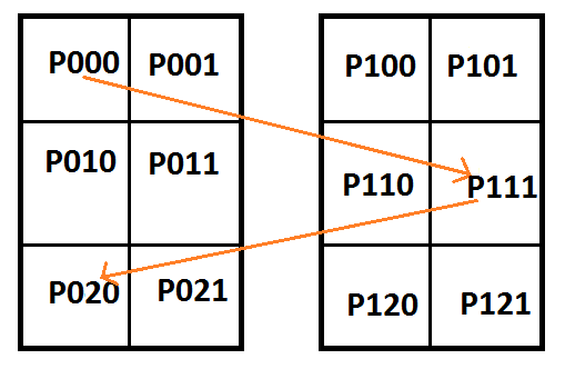
Since the regular 3d texture / cubic curve pattern has a limit (3 curves), let’s look at the C0 continuity version like we did for the 2d texture / quadratic case where we sample zig zag style.
Since the sampling has to pass through the center of the cube, we need to flip both x and z each curve.
That gives us a setup like this:
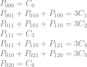
Here are the constraints for the pixel values:
Which looks like this in matrix form:
![\left[\begin{array}{rrrrrrrrrrrr|rrrrrrr} P_{000} & P_{001} & P_{010} & P_{011} & P_{020} & P_{021} & P_{100} & P_{101} & P_{110} & P_{111} & P_{120} & P_{121} & C_{0} & C_{1} & C_{2} & C_{3} & C_{4} & C_{5} & C_{6} \\ 1 & 0 & 0 & 0 & 0 & 0 & 0 & 0 & 0 & 0 & 0 & 0 & 1 & 0 & 0 & 0 & 0 & 0 & 0 \\ 0 & 1 & 1 & 0 & 0 & 0 & 1 & 0 & 0 & 0 & 0 & 0 & 0 & 3 & 0 & 0 & 0 & 0 & 0 \\ 0 & 0 & 0 & 1 & 0 & 0 & 0 & 1 & 1 & 0 & 0 & 0 & 0 & 0 & 3 & 0 & 0 & 0 & 0 \\ 0 & 0 & 0 & 0 & 0 & 0 & 0 & 0 & 0 & 1 & 0 & 0 & 0 & 0 & 0 & 1 & 0 & 0 & 0 \\ 0 & 0 & 0 & 1 & 0 & 0 & 0 & 0 & 1 & 0 & 0 & 1 & 0 & 0 & 0 & 0 & 3 & 0 & 0 \\ 0 & 0 & 1 & 0 & 0 & 1 & 0 & 0 & 0 & 0 & 1 & 0 & 0 & 0 & 0 & 0 & 0 & 3 & 0 \\ 0 & 0 & 0 & 0 & 1 & 0 & 0 & 0 & 0 & 0 & 0 & 0 & 0 & 0 & 0 & 0 & 0 & 0 & 1 \\ \end{array}\right]](https://s0.wp.com/latex.php?latex=%5Cleft%5B%5Cbegin%7Barray%7D%7Brrrrrrrrrrrr%7Crrrrrrr%7D+P_%7B000%7D+%26+P_%7B001%7D+%26+P_%7B010%7D+%26+P_%7B011%7D+%26+P_%7B020%7D+%26+P_%7B021%7D+%26+P_%7B100%7D+%26+P_%7B101%7D+%26+P_%7B110%7D+%26+P_%7B111%7D+%26+P_%7B120%7D+%26+P_%7B121%7D+%26+C_%7B0%7D+%26+C_%7B1%7D+%26+C_%7B2%7D+%26+C_%7B3%7D+%26+C_%7B4%7D+%26+C_%7B5%7D+%26+C_%7B6%7D+%5C%5C+1+%26+0+%26+0+%26+0+%26+0+%26+0+%26+0+%26+0+%26+0+%26+0+%26+0+%26+0+%26+1+%26+0+%26+0+%26+0+%26+0+%26+0+%26+0+%5C%5C+0+%26+1+%26+1+%26+0+%26+0+%26+0+%26+1+%26+0+%26+0+%26+0+%26+0+%26+0+%26+0+%26+3+%26+0+%26+0+%26+0+%26+0+%26+0+%5C%5C+0+%26+0+%26+0+%26+1+%26+0+%26+0+%26+0+%26+1+%26+1+%26+0+%26+0+%26+0+%26+0+%26+0+%26+3+%26+0+%26+0+%26+0+%26+0+%5C%5C+0+%26+0+%26+0+%26+0+%26+0+%26+0+%26+0+%26+0+%26+0+%26+1+%26+0+%26+0+%26+0+%26+0+%26+0+%26+1+%26+0+%26+0+%26+0+%5C%5C+0+%26+0+%26+0+%26+1+%26+0+%26+0+%26+0+%26+0+%26+1+%26+0+%26+0+%26+1+%26+0+%26+0+%26+0+%26+0+%26+3+%26+0+%26+0+%5C%5C+0+%26+0+%26+1+%26+0+%26+0+%26+1+%26+0+%26+0+%26+0+%26+0+%26+1+%26+0+%26+0+%26+0+%26+0+%26+0+%26+0+%26+3+%26+0+%5C%5C+0+%26+0+%26+0+%26+0+%26+1+%26+0+%26+0+%26+0+%26+0+%26+0+%26+0+%26+0+%26+0+%26+0+%26+0+%26+0+%26+0+%26+0+%26+1+%5C%5C+%5Cend%7Barray%7D%5Cright%5D+&bg=ffffff&fg=666666&s=0&c=20201002)
Here is the matrix solved in rref:
![\left[\begin{array}{rrrrrrrrrrrr|rrrrrrr} P_{000} & P_{001} & P_{010} & P_{011} & P_{020} & P_{021} & P_{100} & P_{101} & P_{110} & P_{111} & P_{120} & P_{121} & C_{0} & C_{1} & C_{2} & C_{3} & C_{4} & C_{5} & C_{6} \\ 1 & 0 & 0 & 0 & 0 & 0 & 0 & 0 & 0 & 0 & 0 & 0 & 1 & 0 & 0 & 0 & 0 & 0 & 0 \\ 0 & 1 & 0 & 0 & 0 & -1 & 1 & 0 & 0 & 0 & -1 & 0 & 0 & 3 & 0 & 0 & 0 & -3 & 0 \\ 0 & 0 & 1 & 0 & 0 & 1 & 0 & 0 & 0 & 0 & 1 & 0 & 0 & 0 & 0 & 0 & 0 & 3 & 0 \\ 0 & 0 & 0 & 1 & 0 & 0 & 0 & 0 & 1 & 0 & 0 & 1 & 0 & 0 & 0 & 0 & 3 & 0 & 0 \\ 0 & 0 & 0 & 0 & 1 & 0 & 0 & 0 & 0 & 0 & 0 & 0 & 0 & 0 & 0 & 0 & 0 & 0 & 1 \\ 0 & 0 & 0 & 0 & 0 & 0 & 0 & 1 & 0 & 0 & 0 & -1 & 0 & 0 & 3 & 0 & -3 & 0 & 0 \\ 0 & 0 & 0 & 0 & 0 & 0 & 0 & 0 & 0 & 1 & 0 & 0 & 0 & 0 & 0 & 1 & 0 & 0 & 0 \\ \end{array}\right]](https://s0.wp.com/latex.php?latex=%5Cleft%5B%5Cbegin%7Barray%7D%7Brrrrrrrrrrrr%7Crrrrrrr%7D+P_%7B000%7D+%26+P_%7B001%7D+%26+P_%7B010%7D+%26+P_%7B011%7D+%26+P_%7B020%7D+%26+P_%7B021%7D+%26+P_%7B100%7D+%26+P_%7B101%7D+%26+P_%7B110%7D+%26+P_%7B111%7D+%26+P_%7B120%7D+%26+P_%7B121%7D+%26+C_%7B0%7D+%26+C_%7B1%7D+%26+C_%7B2%7D+%26+C_%7B3%7D+%26+C_%7B4%7D+%26+C_%7B5%7D+%26+C_%7B6%7D+%5C%5C+1+%26+0+%26+0+%26+0+%26+0+%26+0+%26+0+%26+0+%26+0+%26+0+%26+0+%26+0+%26+1+%26+0+%26+0+%26+0+%26+0+%26+0+%26+0+%5C%5C+0+%26+1+%26+0+%26+0+%26+0+%26+-1+%26+1+%26+0+%26+0+%26+0+%26+-1+%26+0+%26+0+%26+3+%26+0+%26+0+%26+0+%26+-3+%26+0+%5C%5C+0+%26+0+%26+1+%26+0+%26+0+%26+1+%26+0+%26+0+%26+0+%26+0+%26+1+%26+0+%26+0+%26+0+%26+0+%26+0+%26+0+%26+3+%26+0+%5C%5C+0+%26+0+%26+0+%26+1+%26+0+%26+0+%26+0+%26+0+%26+1+%26+0+%26+0+%26+1+%26+0+%26+0+%26+0+%26+0+%26+3+%26+0+%26+0+%5C%5C+0+%26+0+%26+0+%26+0+%26+1+%26+0+%26+0+%26+0+%26+0+%26+0+%26+0+%26+0+%26+0+%26+0+%26+0+%26+0+%26+0+%26+0+%26+1+%5C%5C+0+%26+0+%26+0+%26+0+%26+0+%26+0+%26+0+%26+1+%26+0+%26+0+%26+0+%26+-1+%26+0+%26+0+%26+3+%26+0+%26+-3+%26+0+%26+0+%5C%5C+0+%26+0+%26+0+%26+0+%26+0+%26+0+%26+0+%26+0+%26+0+%26+1+%26+0+%26+0+%26+0+%26+0+%26+0+%26+1+%26+0+%26+0+%26+0+%5C%5C+%5Cend%7Barray%7D%5Cright%5D+&bg=ffffff&fg=666666&s=0&c=20201002)
And here is that matrix put back into equations form:

It worked! It also has 5 free variables.
This pattern works for as many curves as i tried (21 of them), and each time you add another curve / row of this pattern you gain another free variable.
So, storing 2 curves results in 6 free variables, 3 curves has 7 free variables, 4 curves has 8 free variables and so on.
9. 3D Texture / Cubic Piecewise Curves – Storage Efficiency
Let’s compare storage efficiency of these 3d texture / cubic curve techniques like we did for the 2d texture / quadratic curve techniques.

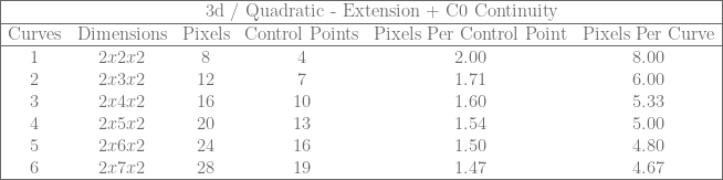

The original technique had a constant 2 pixels per control point and 8 pixels per cubic curve.
The basic extension lets you bring that down to 1.33 pixels per control point, and 5.33 pixels per curve.
If C0 continuity is desired, as you store more and more curves the extension can bring things down towards 1.33 pixels per control point, and 4 pixels per curve. (Remember that with the C0 extension you have 4 control points for the first curve and then 3 more for each subsequent curve, so that 1.33 pixels per control point isn’t exactly an apples to apples comparison vs the basic extension).
The pattern continues for 4D textures and higher (for higher than cubic curves too!), but working through the 2d and 3d cases for quadratic / cubic curves is the most likely usage case both because 4d textures and higher are kind of excessive (probably you’d need to do multiple texture reads to simulate them), but also when fitting curves to data, quadratic and cubic curves tend to do well in that they don’t usually overfit the data or have as many problems with ringing.
Despite that, I do think it’s useful to look at it from an N dimensional point of view to see the larger picture, so let’s do that next.
10. Generalizing The Unit Hyper Cube
Let’s ignore the zig zag sampling pattern and storing multiple curves in a texture and just get back to the basic idea.
Given an N dimensional texture that is 2x2x…x2 that you are going to sample across the diagonal to get a degree N Bezier curve from, how do you know what values to put in which control points to use this technique?
You could derive it from N-linear interpolation, but that is a lot of work.
The good news is it turns out there is a simple pattern, that is also pretty interesting.
Let’s check out the 1d, 2d and 3d cases to see what patterns we might be able to see.
1d Texture / linear Bezier / linear interpolation:

![\left[\begin{array}{rr|rr} P_{0} & P_{1} & C_0 & C_1\\ 1 & 0 & 1 & 0 \\ 0 & 1 & 0 & 1 \\ \end{array}\right]](https://s0.wp.com/latex.php?latex=%5Cleft%5B%5Cbegin%7Barray%7D%7Brr%7Crr%7D+P_%7B0%7D+%26+P_%7B1%7D+%26+C_0+%26+C_1%5C%5C+1+%26+0+%26+1+%26+0+%5C%5C+0+%26+1+%26+0+%26+1+%5C%5C+%5Cend%7Barray%7D%5Cright%5D+&bg=ffffff&fg=666666&s=0&c=20201002)
2d Texture / Quadratic Bezier:
3d Texture / Cubic Bezier:
The first pattern you might see is that the right side of the equations for an N dimensional hypercube is the identity matrix, but instead of using 1 for the value along the diagonal, it uses values from Pascal’s Triangle (binomial coefficients).
To simplify this a bit though, we could also notice that the number on the right side of the equation equals the sum of the numbers on the left side of the equation. Mathematically it would be the same to say that the numbers on the left side of the equation have to sum up to 1. This would make the matrix on the right just be the identity matrix and we can forget about Pascal’s triangle numbers (they will show up implicitly as divisors of the left side equation coefficients but there’s no need to explicitly calculate them).
But then we are still left with the matrix on the left. How do we know which pixels belong in which rows?
It turns out there is another interesting pattern here. In all the matrices above it follows this pattern:
- Row 0 has a “1” wherever the pixel coordinate has 0 ones set
- Row 1 has a “1” wherever the pixel coordinate has 1 ones set
- Row 2 has a “1” wherever the pixel coordinate has 2 ones set
- Row 3 has a “1” wherever the pixel coordinate has 3 ones set
- ….
That pattern continues indefinitely, but don’t forget that the numbers (coefficients) on the left side of the equation must add up to one.
Here is the matrix form of 1d / linear, 2d / quadratic, and 3d / cubic again with the right matrix being the identity matrix, and the equations below them. Notice the pattern about counts of one bits in each row!
1D:

2D:
![\left[\begin{array}{rrrr|rrr} P_{00} & P_{01} & P_{10} & P_{11} & C_0 & C_1 & C_2 \\ 1 & 0 & 0 & 0 & 1 & 0 & 0 \\ 0 & \frac{1}{2} & \frac{1}{2} & 0 & 0 & 1 & 0\\ 0 & 0 & 0 & 1 & 0 & 0 & 1 \end{array}\right]](https://s0.wp.com/latex.php?latex=%5Cleft%5B%5Cbegin%7Barray%7D%7Brrrr%7Crrr%7D+P_%7B00%7D+%26+P_%7B01%7D+%26+P_%7B10%7D+%26+P_%7B11%7D+%26+C_0+%26+C_1+%26+C_2+%5C%5C+1+%26+0+%26+0+%26+0+%26+1+%26+0+%26+0+%5C%5C+0+%26+%5Cfrac%7B1%7D%7B2%7D+%26+%5Cfrac%7B1%7D%7B2%7D+%26+0+%26+0+%26+1+%26+0%5C%5C+0+%26+0+%26+0+%26+1+%26+0+%26+0+%26+1+%5Cend%7Barray%7D%5Cright%5D+&bg=ffffff&fg=666666&s=0&c=20201002)

3D:
![\left[\begin{array}{rrrrrrrr|rrrr} P_{000} & P_{001} & P_{010} & P_{011} & P_{100} & P_{101} & P_{110} & P_{111} & C_0 & C_1 & C_2 & C_3 \\ 1 & 0 & 0 & 0 & 0 & 0 & 0 & 0 & 1 & 0 & 0 & 0 \\ 0 & \frac{1}{3} & \frac{1}{3} & 0 & \frac{1}{3} & 0 & 0 & 0 & 0 & 1 & 0 & 0 \\ 0 & 0 & 0 & \frac{1}{3} & 0 & \frac{1}{3} & \frac{1}{3} & 0 & 0 & 0 & 1 & 0 \\ 0 & 0 & 0 & 0 & 0 & 0 & 0 & 1 & 0 & 0 & 0 & 1 \\ \end{array}\right]](https://s0.wp.com/latex.php?latex=%5Cleft%5B%5Cbegin%7Barray%7D%7Brrrrrrrr%7Crrrr%7D+P_%7B000%7D+%26+P_%7B001%7D+%26+P_%7B010%7D+%26+P_%7B011%7D+%26+P_%7B100%7D+%26+P_%7B101%7D+%26+P_%7B110%7D+%26+P_%7B111%7D+%26++++C_0+%26+C_1+%26+C_2+%26+C_3+%5C%5C+1+%26+0+%26+0+%26+0+%26+0+%26+0+%26+0+%26+0+%26++++1+%26+0+%26+0+%26+0+%5C%5C+0+%26+%5Cfrac%7B1%7D%7B3%7D+%26+%5Cfrac%7B1%7D%7B3%7D+%26+0+%26+%5Cfrac%7B1%7D%7B3%7D+%26+0+%26+0+%26+0+%26++++0+%26+1+%26+0+%26+0+%5C%5C+0+%26+0+%26+0+%26+%5Cfrac%7B1%7D%7B3%7D+%26+0+%26+%5Cfrac%7B1%7D%7B3%7D+%26+%5Cfrac%7B1%7D%7B3%7D+%26+0+%26++++0+%26+0+%26+1+%26+0+%5C%5C+0+%26+0+%26+0+%26+0+%26+0+%26+0+%26+0+%26+1+%26++++0+%26+0+%26+0+%26+1+%5C%5C+%5Cend%7Barray%7D%5Cright%5D+&bg=ffffff&fg=666666&s=0&c=20201002)

Here are the formulas for linear, quadratic and cubic Bezier curves to show a different way of looking at this. Below each is the same formula but with the 1d, 2d and 3d pixels in the formula instead of the control points, using the formulas above which relate pixel values to control point values. Note that I have replaced (1-t) with s for easier reading.


I think it’s really interesting how in the last equation as an example, “3B” literally becomes 3 values which could have the value of B. In the plain vanilla technique they did have the value of B. In this extension, the only requirement is that they average to B.
It’s also interesting to notice that if you have an N bit number and you count how many permutations have each possible number of bits turned on, the resulting counts is the Pascal’s triangle row. That is nothing new, but it seems like there might be a fun way to convert a set of random numbers (white noise) into a Gaussian distribution, just by counting how many one bits there were in each number. That isn’t new either, and there are better algorithms, but still I think it’s an interesting idea, and may be useful in a pinch since it seems pretty computationally inexpensive.
11. Closing
This extension makes storage efficiency a bit better than the plain vanilla technique, especially if you are interested in C0 continuous curves.
The extension does come at a price though, as you may find yourself in a situation where you need to store a value that is outside of the possible values for common data formats to store (such as needing to store a negative number or a larger than 255 number in a uint8).
Even so, if these three criteria are met:
- You are already storing data in textures. (Counter point: compute is usually preferred over texture lookup these days)
- You are relying on the texture interpolator to interpolate values between data points. (Counter point: if you don’t want the interpolation, use a buffer instead so you fit more of the data you actually care about in the cache)
- You are storing data in 16 or 32 bit real numbers. (Counter point: uint8 is half as large as 16 bit and a quarter as large as 32 bit already)
Then this may be an attractive solution for you, even over the plain vanilla technique.
For future work, I think it would be interesting to see how this line of thinking applies to surfaces.
I also think there is probably some fertile ground looking into what happens when sampling off of the diagonal of the textures. Intuitively it seems you might be able to store some special case higher order curves in lower dimension / storage textures, but I haven’t looked into it yet.
A common usage case when encoding data in a texture would probably include putting curves side by side on the x axis of the texture. It could be interesting to look into whether curves need to be completely separate from each other horizontally (aka 2 pixel of width for each track of curves in the texture), or if you could perhaps fit two curves side by side in a 3 pixel width, or any similar ideas.
Lastly, when looking at these groups of points on these N dimensional hyper-cubes, I can’t help but wonder what kinds of shapes they are. Are they simplices? If so, is there a pattern to the dimensions they are of?
It’s a bit hard to visualize, but taking a look at the first few rows of pascal’s triangle / hyper cubes here’s what I found:
- Dimension 1 (line) : Row 2 = 1,1. Those are both points, so are simplices of 0 dimension.
- Dimension 2 (square) : Row 3 = 1,2,1. The 1’s are points, the 2 is a line, so are simplices of dimension 0, 1, 0.
- Dimension 3 (cube) : Row 4 = 1,3,3,1. The 1’s are still points. The 3’s are in fact triangles, I checked. So, simplices of dimension 0, 2, 2, 0.
- Dimension 4 (hypercube) : Row 5 = 1,4,6,4,1. The 1’s are points. The 4’s are tetrahedrons. The 6 is a 3 dimensional object. I’m not sure it’s shape but that makes it not be a simplex. Possibly it’s two simplices fused together some how. I don’t really know. So, the dimensions anyways are: 0, 3, 3, 3, 0.
- Beyond? That’s as far as I looked. If you look further / deeper and find anything interesting please share!
Update: PBS Infinite Series ended up posting a video on the topic of hypercube slices and pascal’s triangle (seriously!). Give it a watch if you are interested in how these things relate: Dissecting Hypercubes with Pascal’s Triangle | Infinite Series
Questions, comments, corrections, etc? Post a comment below or hit me up on twitter at @Atrix256.
If you have a usage case for this or any of the related techniques, I’d love to hear about them.
Thanks for reading!
12. Code
It’s easy to talk about things and claim that everything is correct, when in fact, the moment you try it, everything falls apart.
I made up some simple standalone c++ code that goes through the cases we talked about, doing the math we did, and also verifying that the texture interpolation is equivalent to actually calculating Bezier curves (using Bernstein polynomials).
You can also use this code as a starting point to explore higher curve counts or other storage patterns. It uses only standard includes and no libraries, so it should be real easy to drop this into a compiler and start experimenting.
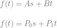
Here’s some example output, which shows 6 cubic curves stored in a 3d texture using the zig zag sampling pattern.
Here’s the code:
#define _CRT_SECURE_NO_WARNINGS

#include <stdio.h>
#include <stdlib.h>
#include <array>
#include <algorithm>
#include <unordered_set>
#include <random>
#include <vector>

#define SHOW_MATHJAX_MATRIX() 0
#define SHOW_MATHJAX_EQUATIONS() 0
#define SHOW_EQUATIONS_BEFORE_SOLVE() 0
#define EQUALITY_TEST_SAMPLES 1000

typedef int32_t TINT;

TINT CalculateGCD (TINT smaller, TINT larger);
TINT CalculateLCM (TINT smaller, TINT larger);

// A rational number, to handle fractional numbers without typical floating point issues
struct CRationalNumber
{
	CRationalNumber (TINT numerator = 0, TINT denominator = 1)
		: m_numerator(numerator)
		, m_denominator(denominator)
	{ }

	TINT m_numerator;
	TINT m_denominator;

	CRationalNumber Reciprocal () const
	{
		return CRationalNumber(m_denominator, m_numerator);
	}

	void Reduce ()
	{
		if (m_numerator != 0 && m_denominator != 0)
		{
			TINT div = CalculateGCD(m_numerator, m_denominator);
			m_numerator /= div;
			m_denominator /= div;
		}

		if (m_denominator < 0)
		{
			m_numerator *= -1;
			m_denominator *= -1;
		}

		if (m_numerator == 0)
			m_denominator = 1;
	}

	bool IsZero () const
	{
		return m_numerator == 0 && m_denominator != 0;
	}

	// NOTE: the functions below assume Reduce() has happened
	bool IsOne () const
	{
		return m_numerator == 1 && m_denominator == 1;
	}

	bool IsMinusOne () const
	{
		return m_numerator == -1 && m_denominator == 1;
	}

	bool IsWholeNumber () const
	{
		return m_denominator == 1;
	}
};

// Define a vector as an array of rational numbers
template<size_t N>
using TVector = std::array<CRationalNumber, N>;

// Define a matrix as an array of vectors
template<size_t M, size_t N>
using TMatrix = std::array<TVector<N>, M>;

//===================================================================================================================================
//                                              GCD / LCM
//===================================================================================================================================

// from my blog post: https://blog.demofox.org/2015/01/24/programmatically-calculating-gcd-and-lcm/

TINT CalculateGCD (TINT smaller, TINT larger)
{
	// make sure A <= B before starting
	if (larger < smaller)
		std::swap(smaller, larger);

	// loop
	while (1)
	{
		// if the remainder of larger / smaller is 0, they are the same
		// so return smaller as the GCD
		TINT remainder = larger % smaller;
		if (remainder == 0)
			return smaller;

		// otherwise, the new larger number is the old smaller number, and
		// the new smaller number is the remainder
		larger = smaller;
		smaller = remainder;
	}
}

TINT CalculateLCM (TINT A, TINT B)
{
	// LCM(A,B) = (A/GCD(A,B))*B
	return (A / CalculateGCD(A, B))*B;
}

//===================================================================================================================================
//                                              RATIONAL NUMBER MATH
//===================================================================================================================================

void CommonDenominators (CRationalNumber& a, CRationalNumber& b)
{
	TINT lcm = CalculateLCM(a.m_denominator, b.m_denominator);

	a.m_numerator *= lcm / a.m_denominator;
	b.m_numerator *= lcm / b.m_denominator;

	a.m_denominator = lcm;
	b.m_denominator = lcm;
}

bool operator == (const CRationalNumber& a, const CRationalNumber& b)
{
	CRationalNumber _a(a), _b(b);
	CommonDenominators(_a, _b);
	return _a.m_numerator == _b.m_numerator;
}

void operator *= (CRationalNumber& a, const CRationalNumber& b)
{
	a.m_numerator *= b.m_numerator;
	a.m_denominator *= b.m_denominator;
}

CRationalNumber operator * (const CRationalNumber& a, const CRationalNumber& b)
{
	return CRationalNumber(a.m_numerator * b.m_numerator, a.m_denominator * b.m_denominator);
}

void operator -= (CRationalNumber& a, const CRationalNumber& b)
{
	CRationalNumber _b(b);
	CommonDenominators(a, _b);
	a.m_numerator -= _b.m_numerator;
}

//===================================================================================================================================
//                                              GAUSS-JORDAN ELIMINATION CODE
//===================================================================================================================================

// From my blog post: https://blog.demofox.org/2017/04/10/solving-n-equations-and-n-unknowns-the-fine-print-gauss-jordan-elimination/

// Make a specific row have a 1 in the colIndex, and make all other rows have 0 there
template <size_t M, size_t N>
bool MakeRowClaimVariable (TMatrix<M, N>& matrix, size_t rowIndex, size_t colIndex)
{
    // Find a row that has a non zero value in this column and swap it with this row
    {
        // Find a row that has a non zero value
        size_t nonZeroRowIndex = rowIndex;
        while (nonZeroRowIndex < M && matrix[nonZeroRowIndex][colIndex].IsZero())
            ++nonZeroRowIndex;

        // If there isn't one, nothing to do
        if (nonZeroRowIndex == M)
            return false;

        // Otherwise, swap the row
        if (rowIndex != nonZeroRowIndex)
            std::swap(matrix[rowIndex], matrix[nonZeroRowIndex]);
    }

    // Scale this row so that it has a leading one
    CRationalNumber scale = matrix[rowIndex][colIndex].Reciprocal();
	for (size_t normalizeColIndex = colIndex; normalizeColIndex < N; ++normalizeColIndex)
	{
		matrix[rowIndex][normalizeColIndex] *= scale;
		matrix[rowIndex][normalizeColIndex].Reduce();
	}

    // Make sure all rows except this one have a zero in this column.
    // Do this by subtracting this row from other rows, multiplied by a multiple that makes the column disappear.
    for (size_t eliminateRowIndex = 0; eliminateRowIndex < M; ++eliminateRowIndex)
    {
        if (eliminateRowIndex == rowIndex)
            continue;

        CRationalNumber scale = matrix[eliminateRowIndex][colIndex];
		for (size_t eliminateColIndex = 0; eliminateColIndex < N; ++eliminateColIndex)
		{
			matrix[eliminateRowIndex][eliminateColIndex] -= matrix[rowIndex][eliminateColIndex] * scale;
			matrix[eliminateRowIndex][eliminateColIndex].Reduce();
		}
    }

    return true;
}

// make matrix into reduced row echelon form
template <size_t M, size_t N>
void GaussJordanElimination (TMatrix<M, N>& matrix)
{
    size_t rowIndex = 0;
    for (size_t colIndex = 0; colIndex < N; ++colIndex)
    {
        if (MakeRowClaimVariable(matrix, rowIndex, colIndex))
        {
            ++rowIndex;
            if (rowIndex == M)
                return;
        }
    }
}

//===================================================================================================================================
//                                                           Shared Testing Code
//===================================================================================================================================

template <size_t M, size_t N, typename LAMBDA>
void PrintEquations (
	TMatrix<M, N>& augmentedMatrix,
	size_t numPixels,
	LAMBDA& pixelIndexToCoordinates
)
{
	char pixelCoords[10];

#if SHOW_MATHJAX_MATRIX()
	// print the matrix opening stuff
	printf("\left[\begin{array}{");
	for (size_t i = 0; i < N; ++i)
	{
		if (i == numPixels)
			printf("|");
		printf("r");
	}
	printf("}n");
	// print the header row
	for (size_t i = 0; i < numPixels; ++i)
	{
		pixelIndexToCoordinates(i, pixelCoords);
		if (i == 0)
			printf("P_{%s}", pixelCoords);
		else
			printf(" & P_{%s}", pixelCoords);
	}
	for (size_t i = numPixels; i < N; ++i)
	{
		printf(" & C_{%zu}", i-numPixels);
	}
	printf(" \\n");

	// Print the matrix
	for (const TVector<N>& row : augmentedMatrix)
	{
		bool first = true;
		for (const CRationalNumber& n : row)
		{
			if (first)
				first = false;
			else
				printf(" & ");

			if (n.IsWholeNumber())
				printf("%i", n.m_numerator);
			else
				printf("\frac{%i}{%i}", n.m_numerator, n.m_denominator);
		}
		printf(" \\n");
	}

	// print the matrix closing stuff
	printf("\end{array}\right]n");
#endif

	// print equations
	for (const TVector<N>& row : augmentedMatrix)
	{
		// indent
		#if SHOW_MATHJAX_EQUATIONS() == 0
			printf("    ");
		#endif

		// left side of the equation
		bool leftHasATerm = false;
		for (size_t i = 0; i < numPixels; ++i)
		{
			if (!row[i].IsZero())
			{
				if (leftHasATerm)
					printf(" + ");
				pixelIndexToCoordinates(i, pixelCoords);

				#if SHOW_MATHJAX_EQUATIONS()
					if (row[i].IsOne())
						printf("P_{%s}", pixelCoords);
					else if (row[i].IsMinusOne())
						printf("-P_{%s}", pixelCoords);
					else if (row[i].IsWholeNumber())
						printf("%iP_{%s}", row[i].m_numerator, pixelCoords);
					else if (row[i].m_numerator == 1)
						printf("P_{%s}/%i", pixelCoords, row[i].m_denominator);
					else
						printf("P_{%s} * %i/%i", pixelCoords, row[i].m_numerator, row[i].m_denominator);
				#else
					if (row[i].IsOne())
						printf("P%s", pixelCoords);
					else if (row[i].IsMinusOne())
						printf("-P%s", pixelCoords);
					else if (row[i].IsWholeNumber())
						printf("%iP%s", row[i].m_numerator, pixelCoords);
					else if (row[i].m_numerator == 1)
						printf("P%s/%i", pixelCoords, row[i].m_denominator);
					else
						printf("P%s * %i/%i", pixelCoords, row[i].m_numerator, row[i].m_denominator);
				#endif
				leftHasATerm = true;
			}
		}
		if (!leftHasATerm)
			printf("0 = ");
		else
			printf(" = ");

		// right side of the equation
		bool rightHasATerm = false;
		for (size_t i = numPixels; i < N; ++i)
		{
			if (!row[i].IsZero())
			{
				if (rightHasATerm)
					printf(" + ");

				#if SHOW_MATHJAX_EQUATIONS()
					if (row[i].IsOne())
						printf("C_{%zu}", i - numPixels);
					else if (row[i].IsMinusOne())
						printf("-C_{%zu}", i - numPixels);
					else if (row[i].IsWholeNumber())
						printf("%iC_{%zu}", row[i].m_numerator, i - numPixels);
					else if (row[i].m_numerator == 1)
						printf("C_{%zu}/%i", i - numPixels, row[i].m_denominator);
					else
						printf("C_{%zu} * %i/%i", i - numPixels, row[i].m_numerator, row[i].m_denominator);
				#else
					if (row[i].IsOne())
						printf("C%zu", i - numPixels);
					else if (row[i].IsMinusOne())
						printf("-C%zu", i - numPixels);
					else if (row[i].IsWholeNumber())
						printf("%iC%zu", row[i].m_numerator, i - numPixels);
					else if (row[i].m_numerator == 1)
						printf("C%zu/%i", i - numPixels, row[i].m_denominator);
					else
						printf("C%zu * %i/%i", i - numPixels, row[i].m_numerator, row[i].m_denominator);
				#endif
				rightHasATerm = true;
			}
		}

		#if SHOW_MATHJAX_EQUATIONS()
			printf("\\n");
		#else
			printf("n");
		#endif
	}
}

template <size_t M, size_t N, typename LAMBDA>
bool SolveMatrixAndPrintEquations (
	TMatrix<M, N>& augmentedMatrix,
	size_t numPixels,
	std::unordered_set<size_t>& freeVariables,
	LAMBDA& pixelIndexToCoordinates
)
{
	#if SHOW_EQUATIONS_BEFORE_SOLVE()
	printf("   Initial Equations:n");
	PrintEquations(augmentedMatrix, numPixels, pixelIndexToCoordinates);
	printf("   Solved Equations:n");
	#endif

	// put augmented matrix into rref
	GaussJordanElimination(augmentedMatrix);

	// Print equations
	PrintEquations(augmentedMatrix, numPixels, pixelIndexToCoordinates);

	// Get free variables and check for control point constraint
	bool constraintFound = false;
	for (const TVector<N>& row : augmentedMatrix)
	{
		bool leftHasATerm = false;
		for (size_t i = 0; i < numPixels; ++i)
		{
			if (!row[i].IsZero())
			{
				if (leftHasATerm)
					freeVariables.insert(i);
				else
					leftHasATerm = true;
			}
		}

		bool rightHasATerm = false;
		for (size_t i = numPixels; i < N; ++i)
		{
			if (!row[i].IsZero())
				rightHasATerm = true;
		}

		if (!leftHasATerm && rightHasATerm)
			constraintFound = true;
	}

	printf("  %zu free variables.n", freeVariables.size());

	if (constraintFound)
	{
		printf("  Constraint Found.  This configuration doesn't work for the general case!nn");
		return false;
	}

	return true;
}

float lerp (float t, float a, float b)
{
	return a * (1.0f - t) + b * t;
}

template <size_t NUMPIXELS, size_t NUMCONTROLPOINTS, size_t NUMEQUATIONS>
void FillInPixelsAndControlPoints (
	std::array<float, NUMPIXELS>& pixels,
	std::array<float, NUMCONTROLPOINTS>& controlPoints,
	const TMatrix<NUMEQUATIONS, NUMPIXELS+ NUMCONTROLPOINTS>& augmentedMatrix,
	const std::unordered_set<size_t>& freeVariables)
{
	// come up with random values for the control points and free variable pixels
	static std::random_device rd;
	static std::mt19937 mt(rd());
	static std::uniform_real_distribution<float> dist(-10.0f, 10.0f);
	for (float& cp : controlPoints)
		cp = dist(mt);
	for (size_t var : freeVariables)
		pixels[var] = dist(mt);

	// fill in the non free variable pixels per the equations
	for (const TVector<NUMPIXELS + NUMCONTROLPOINTS>& row : augmentedMatrix)
	{
		// the first non zero value is the non free pixel we need to set.
		// all other non zero values are free variables that we previously calculated values for
		bool foundPixel = false;
		size_t pixelIndex = 0;
		for (size_t i = 0; i < NUMPIXELS; ++i)
		{
			if (!row[i].IsZero())
			{
				// we are setting the first pixel we find
				if (!foundPixel)
				{
					pixelIndex = i;
					foundPixel = true;
				}
				// subtract out all free variables which is the same as moving them to the right side of the equation
				else
				{
					pixels[pixelIndex] -= pixels[i] * float(row[i].m_numerator) / float(row[i].m_denominator);
				}
			}
		}

		// if there is no pixel value to set on the left side of the equation, ignore this row
		if (!foundPixel)
			continue;

		// add in the values from the right side of the equation
		for (size_t i = NUMPIXELS; i < NUMPIXELS + NUMCONTROLPOINTS; ++i)
		{
			if (!row[i].IsZero())
				pixels[pixelIndex] += controlPoints[i - NUMPIXELS] * float(row[i].m_numerator) / float(row[i].m_denominator);
		}
	}
}

size_t TextureCoordinateToPixelIndex2d (size_t width, size_t height, size_t y, size_t x)
{
	return y * width + x;
};

void PixelIndexToTextureCoordinate2d (size_t width, size_t height, size_t pixelIndex, size_t& y, size_t& x)
{
	x = pixelIndex % width;
	y = pixelIndex / width;
}

size_t TextureCoordinateToPixelIndex3d (size_t width, size_t height, size_t depth, size_t z, size_t y, size_t x)
{
	return
		z * width * height +
		y * width +
		x;
};

void PixelIndexToTextureCoordinate3d (size_t width, size_t height, size_t depth, size_t pixelIndex, size_t& z, size_t& y, size_t& x)
{
	x = pixelIndex % width;

	pixelIndex = pixelIndex / width;

	y = pixelIndex % height;

	pixelIndex = pixelIndex / height;

	z = pixelIndex;
}

void PiecewiseCurveTime (float time, size_t numCurves, size_t& outCurveIndex, float& outTime)
{
	time *= float(numCurves);
	outCurveIndex = size_t(time);

	if (outCurveIndex == numCurves)
	{
		outCurveIndex = numCurves - 1;
		outTime = 1.0f;
	}
	else
	{
		outTime = std::fmodf(time, 1.0f);
	}
}


//===================================================================================================================================
//                                                       2D Textures / Quadratic Curves
//===================================================================================================================================
//
// Find the limitations of this pattern and show equivalence to Bernstein Polynomials (Bezier Curve Equations). Pattern details below.
//
//  --- For first curve, do:
//
//  P00 P01
//  P10 P11
//
//  P00 = C0                        0
//  P01 + P10 = 2 * C1              1 2
//  P11 = C2                        3
//
//  --- For each additional curve, add two points to the end like this:
//
//  P00 P01
//  P10 P11
//  P20 P21
//
//  P00 = C0                        0
//  P01 + P10 = 2 * C1              1 2
//  P11 = C2                        3
//
//  P10 = C3                        1
//  P11 + P20 = 2 * C4              3 4
//  P21 = C5                        5
//
//  and so on...
//  each equation is then multiplied by a value so the right side is identity and left side coefficients add up to 1.
//
//  --- Other details:
//
//  * 3 control points per curve.
//  * image width it 2
//  * image height is 1 + NumCurves.
//  * there are 3 equations per curve, so 3 rows in the augmented matrix per curve.
//  * augmented matrix columns = num pixels (left columns) + num control points (right columns)
//

template <size_t N>
float EvaluateBernsteinPolynomial2DQuadratic (float totalTime, const std::array<float, N>& coefficients)
{
	const size_t c_numCurves = N / 3;

	float t;
	size_t startCurve;
	PiecewiseCurveTime(totalTime, c_numCurves, startCurve, t);

	size_t offset = startCurve * 3;

	float s = 1.0f - t;
	return
		coefficients[offset + 0] * s * s +
		coefficients[offset + 1] * s * t * 2.0f +
		coefficients[offset + 2] * t * t;
}

template <size_t N>
float EvaluateLinearInterpolation2DQuadratic (float totalTime, const std::array<float, N>& pixels)
{
	const size_t c_numCurves = (N / 2) - 1;

	float t;
	size_t startRow;
	PiecewiseCurveTime(totalTime, c_numCurves, startRow, t);

	float row0 = lerp(t, pixels[startRow * 2], pixels[startRow * 2 + 1]);
	float row1 = lerp(t, pixels[(startRow + 1) * 2], pixels[(startRow + 1) * 2 + 1]);
	return lerp(t, row0, row1);
}

template <size_t NUMCURVES>
void Test2DQuadratic ()
{
	const size_t c_imageWidth = 2;
	const size_t c_imageHeight = NUMCURVES + 1;
	const size_t c_numPixels = c_imageWidth * c_imageHeight;
	const size_t c_numControlPoints = NUMCURVES * 3;
	const size_t c_numEquations = NUMCURVES * 3;

	// report values for this test
	printf("  %zu curves.  %zu control points.  2x%zu texture = %zu pixels.n", NUMCURVES, c_numControlPoints, c_imageHeight, c_numPixels);
	printf("  %f pixels per curve.  %f pixels per control point.n", float(c_numPixels) / float(NUMCURVES), float(c_numPixels) / float(c_numControlPoints));

	// lambdas to convert between pixel index and texture coordinates
	auto TextureCoordinateToPixelIndex = [&](size_t y, size_t x) -> size_t
	{
		return TextureCoordinateToPixelIndex2d(c_imageWidth, c_imageHeight, y, x);
	};
	auto pixelIndexToCoordinates = [&](size_t pixelIndex, char pixelCoords[10])
	{
		size_t y, x;
		PixelIndexToTextureCoordinate2d(c_imageWidth, c_imageHeight, pixelIndex, y, x);
		sprintf(pixelCoords, "%zu%zu", y, x);
	};

	// create the equations
	TMatrix<c_numEquations, c_numPixels + c_numControlPoints> augmentedMatrix;
	for (size_t i = 0; i < c_numEquations; ++i)
	{
		TVector<c_numPixels + c_numControlPoints>& row = augmentedMatrix[i];

		// left side of the equation goes in this yx coordinate pattern:
		//   00
		//   01 10
		//   11
		// But, curve index is added to the y index.
		// Also, left side coefficients must add up to 1.
		size_t curveIndex = i / 3;
		switch (i % 3)
		{
			case 0:
			{
				row[TextureCoordinateToPixelIndex(curveIndex + 0, 0)] = CRationalNumber(1, 1);
				break;
			}
			case 1:
			{
				row[TextureCoordinateToPixelIndex(curveIndex + 0, 1)] = CRationalNumber(1, 2);
				row[TextureCoordinateToPixelIndex(curveIndex + 1, 0)] = CRationalNumber(1, 2);
				break;
			}
			case 2:
			{
				row[TextureCoordinateToPixelIndex(curveIndex + 1, 1)] = CRationalNumber(1, 1);
				break;
			}
		}

		// right side of the equation is identity
		row[c_numPixels + i] = CRationalNumber(1);
	}

	// solve the matrix if possible and print out the equations
	std::unordered_set<size_t> freeVariables;
	if (!SolveMatrixAndPrintEquations(augmentedMatrix, c_numPixels, freeVariables, pixelIndexToCoordinates))
		return;

	// Next we need to show equality between the N-linear interpolation of our pixels and bernstein polynomials with our control points as coefficients

	// Fill in random values for our control points and free variable pixels, and fill in the other pixels as the equations dictate
	std::array<float, c_numPixels> pixels = { 0 };
	std::array<float, c_numControlPoints> controlPoints = { 0 };
	FillInPixelsAndControlPoints<c_numPixels, c_numControlPoints, c_numEquations>(pixels, controlPoints, augmentedMatrix, freeVariables);

	// do a number of samples of each method at the same time values, and report the largest difference (error)
	float largestDifference = 0.0f;
	for (size_t i = 0; i < EQUALITY_TEST_SAMPLES; ++i)
	{
		float t = float(i) / float(EQUALITY_TEST_SAMPLES - 1);

		float value1 = EvaluateBernsteinPolynomial2DQuadratic(t, controlPoints);
		float value2 = EvaluateLinearInterpolation2DQuadratic(t, pixels);

		largestDifference = std::max(largestDifference, std::abs(value1 - value2));
	}
	printf("  %i Samples, Largest Error = %fnn", EQUALITY_TEST_SAMPLES, largestDifference);
}

void Test2DQuadratics ()
{
	printf("Testing 2D Textures / Quadratic Curvesnn");

	Test2DQuadratic<1>();
	Test2DQuadratic<2>();
	Test2DQuadratic<3>();

	system("pause");
}

//===================================================================================================================================
//                                    2D Textures / Quadratic Curves With C0 Continuity
//===================================================================================================================================
//
// Find the limitations of this pattern and show equivalence to Bernstein Polynomials (Bezier Curve Equations). Pattern details below.
//
//  --- For first curve, do:
//
//  P00 P01
//  P10 P11
//
//  P00 = C0                        0
//  P01 + P10 = 2 * C1              1 2
//  P11 = C2                        3
//
//  --- For second curve, do:
//
//  P00 P01
//  P10 P11
//  P20 P21
//
//  P00 = C0                        0
//  P01 + P10 = 2 * C1              1 2
//  P11 = C2                        3
//
//  P10 + P21 = 2 * C3              2 5
//  P20 = C4                        4
//
//  --- For third curve, do:
//
//  P00 P01
//  P10 P11
//  P20 P21
//  P30 P31
//
//  P00 = C0
//  P01 + P10 = 2 * C1
//  P11 = C2
//
//  P10 + P21 = 2 * C3
//  P20 = C4
//
//  P21 + P30 = 2 * C5
//  P31 = C6
//
//  and so on...
//  each equation is then multiplied by a value so the right side is identity and left side coefficients add up to 1.
//
//  --- Other details:
//
//  * control points: 1 + NumCurves*2.
//  * image width it 2
//  * image height is 1 + NumCurves.
//  * equations: 1 + NumCurves*2.  This many rows in the augmented matrix.
//  * augmented matrix columns = num pixels (left columns) + num control points (right columns)
//

template <size_t N>
float EvaluateBernsteinPolynomial2DQuadraticC0 (float totalTime, const std::array<float, N>& coefficients)
{
	const size_t c_numCurves = (N - 1) / 2;

	float t;
	size_t startCurve;
	PiecewiseCurveTime(totalTime, c_numCurves, startCurve, t);

	size_t offset = startCurve * 2;

	float s = 1.0f - t;
	return
		coefficients[offset + 0] * s * s +
		coefficients[offset + 1] * s * t * 2.0f +
		coefficients[offset + 2] * t * t;
}

template <size_t N>
float EvaluateLinearInterpolation2DQuadraticC0 (float totalTime, const std::array<float, N>& pixels)
{
	const size_t c_numCurves = (N / 2) - 1;

	float t;
	size_t startRow;
	PiecewiseCurveTime(totalTime, c_numCurves, startRow, t);

	// Note we flip x axis direction every odd row to get the zig zag
	float horizT = (startRow % 2) == 0 ? t : 1.0f - t;

	float row0 = lerp(horizT, pixels[startRow * 2], pixels[startRow * 2 + 1]);
	++startRow;
	float row1 = lerp(horizT, pixels[startRow * 2], pixels[startRow * 2 + 1]);
	return lerp(t, row0, row1);
}

template <size_t NUMCURVES>
void Test2DQuadraticC0 ()
{
	const size_t c_imageWidth = 2;
	const size_t c_imageHeight = NUMCURVES + 1;
	const size_t c_numPixels = c_imageWidth * c_imageHeight;
	const size_t c_numControlPoints = 1 + NUMCURVES * 2;
	const size_t c_numEquations = 1 + NUMCURVES * 2;

	// report values for this test
	printf("  %zu curves.  %zu control points.  2x%zu texture = %zu pixels.n", NUMCURVES, c_numControlPoints, c_imageHeight, c_numPixels);
	printf("  %f pixels per curve.  %f pixels per control point.n", float(c_numPixels) / float(NUMCURVES), float(c_numPixels) / float(c_numControlPoints));

	// lambdas to convert between pixel index and texture coordinates
	auto TextureCoordinateToPixelIndex = [&] (size_t y, size_t x) -> size_t
	{
		return TextureCoordinateToPixelIndex2d(c_imageWidth, c_imageHeight, y, x);
	};
	auto pixelIndexToCoordinates = [&] (size_t pixelIndex, char pixelCoords[10])
	{
		size_t y, x;
		PixelIndexToTextureCoordinate2d(c_imageWidth, c_imageHeight, pixelIndex, y, x);
		sprintf(pixelCoords, "%zu%zu", y, x);
	};

	// create the equations
	TMatrix<c_numEquations, c_numPixels + c_numControlPoints> augmentedMatrix;
	for (size_t i = 0; i < c_numEquations; ++i)
	{
		TVector<c_numPixels + c_numControlPoints>& row = augmentedMatrix[i];

		// left side of the equation has a pattern like this:
		//   00
		//   01 10
		//
		// But, pattern index is added to the y index.
		// Also, the x coordinates flip from 0 to 1 on those after each pattern.
		// Also, left side coefficients must add up to 1.

		size_t patternIndex = i / 2;
		size_t xoff = patternIndex % 2 == 1;
		size_t xon = patternIndex % 2 == 0;
		switch (i % 2)
		{
			case 0:
			{
				row[TextureCoordinateToPixelIndex(patternIndex + 0, xoff)] = CRationalNumber(1, 1);
				break;
			}
			case 1:
			{
				row[TextureCoordinateToPixelIndex(patternIndex + 0, xon)] = CRationalNumber(1, 2);
				row[TextureCoordinateToPixelIndex(patternIndex + 1, xoff)] = CRationalNumber(1, 2);
				break;
			}
		}

		// right side of the equation is identity
		row[c_numPixels + i] = CRationalNumber(1);
	}

	// solve the matrix if possible and print out the equations
	std::unordered_set<size_t> freeVariables;
	if (!SolveMatrixAndPrintEquations(augmentedMatrix, c_numPixels, freeVariables, pixelIndexToCoordinates))
		return;

	// Next we need to show equality between the N-linear interpolation of our pixels and bernstein polynomials with our control points as coefficients

	// Fill in random values for our control points and free variable pixels, and fill in the other pixels as the equations dictate
	std::array<float, c_numPixels> pixels = { 0 };
	std::array<float, c_numControlPoints> controlPoints = { 0 };
	FillInPixelsAndControlPoints<c_numPixels, c_numControlPoints, c_numEquations>(pixels, controlPoints, augmentedMatrix, freeVariables);

	// do a number of samples of each method at the same time values, and report the largest difference (error)
	float largestDifference = 0.0f;
	for (size_t i = 0; i < EQUALITY_TEST_SAMPLES; ++i)
	{
		float t = float(i) / float(EQUALITY_TEST_SAMPLES - 1);

		float value1 = EvaluateBernsteinPolynomial2DQuadraticC0(t, controlPoints);
		float value2 = EvaluateLinearInterpolation2DQuadraticC0(t, pixels);

		largestDifference = std::max(largestDifference, std::abs(value1 - value2));
	}
	printf("  %i Samples, Largest Error = %fnn", EQUALITY_TEST_SAMPLES, largestDifference);
}

void Test2DQuadraticsC0 ()
{
	printf("nTesting 2D Textures / Quadratic Curves with C0 continuitynn");

	Test2DQuadraticC0<1>();
	Test2DQuadraticC0<2>();
	Test2DQuadraticC0<3>();
	Test2DQuadraticC0<4>();

	system("pause");
}

//===================================================================================================================================
//                                             3D Textures / Cubic Curves
//===================================================================================================================================
//
// Find the limitations of this pattern and show equivalence to Bernstein Polynomials (Bezier Curve Equations). Pattern details below.
//
//  --- For first curve, do:
//
//  P000 P001    P100 P101
//  P010 P011    P110 P111
//
//  P000 = C0                       0
//  P001 + P010 + P100 = 3 * C1     1 2 4
//  P011 + P101 + P110 = 3 * C2     3 5 6
//  P111 = C3                       7
//
//  --- For second curve, do:
//
//  P000 P001    P100 P101
//  P010 P011    P110 P111
//  P020 P021    P120 P121
//
//  P000 = C0                       0
//  P001 + P010 + P100 = 3 * C1     1 2 4
//  P011 + P101 + P110 = 3 * C2     3 7 8
//  P111 = C3                       9
//
//  P010 = C4                       2
//  P011 + P020 + P110 = 3 * C5     3 4 8
//  P021 + P111 + P120 = 3 * C6     5 9 10
//  P121 = C7                       11
//
//  and so on...
//  each equation is then multiplied by a value so the right side is identity and left side coefficients add up to 1.
//
//  --- Other details:
//
//  * control points: 4 * NumCurves.
//  * image width it 2
//  * image depth is 2
//  * image height is 1 + NumCurves.
//  * equations: 4 * NumCurves.  This many rows in the augmented matrix.
//  * augmented matrix columns = num pixels (left columns) + num control points (right columns)
//

template <size_t N>
float EvaluateBernsteinPolynomial3DCubic (float totalTime, const std::array<float, N>& coefficients)
{
	const size_t c_numCurves = N / 4;

	float t;
	size_t startCurve;
	PiecewiseCurveTime(totalTime, c_numCurves, startCurve, t);

	size_t offset = startCurve * 4;

	float s = 1.0f - t;
	return
		coefficients[offset + 0] * s * s * s +
		coefficients[offset + 1] * s * s * t * 3.0f +
		coefficients[offset + 2] * s * t * t * 3.0f +
		coefficients[offset + 3] * t * t * t;
}

template <size_t N, typename LAMBDA>
float EvaluateLinearInterpolation3DCubic (float totalTime, const std::array<float, N>& pixels, LAMBDA& TextureCoordinateToPixelIndex)
{
	const size_t c_numCurves = (N / 4) - 1;

	float t;
	size_t startRow;
	PiecewiseCurveTime(totalTime, c_numCurves, startRow, t);

	//    rowZYX
	float row00x = lerp(t, pixels[TextureCoordinateToPixelIndex(0, startRow + 0, 0)], pixels[TextureCoordinateToPixelIndex(0, startRow + 0, 1)]);
	float row01x = lerp(t, pixels[TextureCoordinateToPixelIndex(0, startRow + 1, 0)], pixels[TextureCoordinateToPixelIndex(0, startRow + 1, 1)]);
	float row0yx = lerp(t, row00x, row01x);

	float row10x = lerp(t, pixels[TextureCoordinateToPixelIndex(1, startRow + 0, 0)], pixels[TextureCoordinateToPixelIndex(1, startRow + 0, 1)]);
	float row11x = lerp(t, pixels[TextureCoordinateToPixelIndex(1, startRow + 1, 0)], pixels[TextureCoordinateToPixelIndex(1, startRow + 1, 1)]);
	float row1yx = lerp(t, row10x, row11x);

	return lerp(t, row0yx, row1yx);
}

template <size_t NUMCURVES>
void Test3DCubic ()
{
	const size_t c_imageWidth = 2;
	const size_t c_imageHeight = NUMCURVES + 1;
	const size_t c_imageDepth = 2;
	const size_t c_numPixels = c_imageWidth * c_imageHeight * c_imageDepth;
	const size_t c_numControlPoints = NUMCURVES * 4;
	const size_t c_numEquations = NUMCURVES * 4;

	// report values for this test
	printf("  %zu curves.  %zu control points.  2x%zux2 texture = %zu pixels.n", NUMCURVES, c_numControlPoints, c_imageHeight, c_numPixels);
	printf("  %f pixels per curve.  %f pixels per control point.n", float(c_numPixels) / float(NUMCURVES), float(c_numPixels) / float(c_numControlPoints));

	// lambdas to convert between pixel index and texture coordinates
	auto TextureCoordinateToPixelIndex = [&] (size_t z, size_t y, size_t x) -> size_t
	{
		return TextureCoordinateToPixelIndex3d(c_imageWidth, c_imageHeight, c_imageDepth, z, y, x);
	};
	auto pixelIndexToCoordinates = [&] (size_t pixelIndex, char pixelCoords[10])
	{
		size_t z, y, x;
		PixelIndexToTextureCoordinate3d(c_imageWidth, c_imageHeight, c_imageDepth, pixelIndex, z, y, x);
		sprintf(pixelCoords, "%zu%zu%zu", z,y,x);
	};

	// create the equations
	TMatrix<c_numEquations, c_numPixels + c_numControlPoints> augmentedMatrix;
	for (size_t i = 0; i < c_numEquations; ++i)
	{
		TVector<c_numPixels + c_numControlPoints>& row = augmentedMatrix[i];

		// left side of the equation goes in this zyx coordinate pattern:
		//   000
		//   001 010 100
		//   011 101 110
		//   111
		// But, curve index is added to the y index.
		// Also, left side coefficients must add up to 1.
		size_t curveIndex = i / 4;
		switch (i % 4)
		{
			case 0:
			{
				row[TextureCoordinateToPixelIndex(0, curveIndex + 0, 0)] = CRationalNumber(1, 1);
				break;
			}
			case 1:
			{
				row[TextureCoordinateToPixelIndex(0, curveIndex + 0, 1)] = CRationalNumber(1, 3);
				row[TextureCoordinateToPixelIndex(0, curveIndex + 1, 0)] = CRationalNumber(1, 3);
				row[TextureCoordinateToPixelIndex(1, curveIndex + 0, 0)] = CRationalNumber(1, 3);
				break;
			}
			case 2:
			{
				row[TextureCoordinateToPixelIndex(0, curveIndex + 1, 1)] = CRationalNumber(1, 3);
				row[TextureCoordinateToPixelIndex(1, curveIndex + 0, 1)] = CRationalNumber(1, 3);
				row[TextureCoordinateToPixelIndex(1, curveIndex + 1, 0)] = CRationalNumber(1, 3);
				break;
			}
			case 3:
			{
				row[TextureCoordinateToPixelIndex(1, curveIndex + 1, 1)] = CRationalNumber(1, 1);
				break;
			}
		}

		// right side of the equation is identity
		row[c_numPixels + i] = CRationalNumber(1);
	}

	// solve the matrix if possible and print out the equations
	std::unordered_set<size_t> freeVariables;
	if (!SolveMatrixAndPrintEquations(augmentedMatrix, c_numPixels, freeVariables, pixelIndexToCoordinates))
		return;

	// Next we need to show equality between the N-linear interpolation of our pixels and bernstein polynomials with our control points as coefficients

	// Fill in random values for our control points and free variable pixels, and fill in the other pixels as the equations dictate
	std::array<float, c_numPixels> pixels = { 0 };
	std::array<float, c_numControlPoints> controlPoints = { 0 };
	FillInPixelsAndControlPoints<c_numPixels, c_numControlPoints, c_numEquations>(pixels, controlPoints, augmentedMatrix, freeVariables);

	// do a number of samples of each method at the same time values, and report the largest difference (error)
	float largestDifference = 0.0f;
	for (size_t i = 0; i < EQUALITY_TEST_SAMPLES; ++i)
	{
		float t = float(i) / float(EQUALITY_TEST_SAMPLES - 1);

		float value1 = EvaluateBernsteinPolynomial3DCubic(t, controlPoints);
		float value2 = EvaluateLinearInterpolation3DCubic(t, pixels, TextureCoordinateToPixelIndex);

		largestDifference = std::max(largestDifference, std::abs(value1 - value2));
	}
	printf("  %i Samples, Largest Error = %fnn", EQUALITY_TEST_SAMPLES, largestDifference);
}

void Test3DCubics ()
{
	printf("nTesting 3D Textures / Cubic Curvesnn");

	Test3DCubic<1>();
	Test3DCubic<2>();
	Test3DCubic<3>();
	Test3DCubic<4>();

	system("pause");
}

//===================================================================================================================================
//                                         3D Textures / Cubic Curves Multiple Curves
//===================================================================================================================================
//
// Find the limitations of this pattern and show equivalence to Bernstein Polynomials (Bezier Curve Equations). Pattern details below.
//
// This is the same as 3D Textures / Cubic Curves, but there is a second curve stored by flipping x coordinates.
//
//  --- Other details:
//
//  * control points: 4 * NumCurves.
//  * image width it 2
//  * image depth is 2
//  * image height is 1 + (NumCurves/2).
//  * equations: 4 * NumCurves.  This many rows in the augmented matrix.
//  * augmented matrix columns = num pixels (left columns) + num control points (right columns)
//

template <size_t HALFNUMCURVES>
void Test3DCubicMulti ()
{
	const size_t NUMCURVES = HALFNUMCURVES * 2;
	const size_t c_imageWidth = 2;
	const size_t c_imageHeight = HALFNUMCURVES + 1;
	const size_t c_imageDepth = 2;
	const size_t c_numPixels = c_imageWidth * c_imageHeight * c_imageDepth;
	const size_t c_numControlPoints = NUMCURVES * 4;
	const size_t c_numEquations = NUMCURVES * 4;

	// report values for this test
	printf("  %zu curves.  %zu control points.  2x%zux2 texture = %zu pixels.n", NUMCURVES, c_numControlPoints, c_imageHeight, c_numPixels);
	printf("  %f pixels per curve.  %f pixels per control point.n", float(c_numPixels) / float(NUMCURVES), float(c_numPixels) / float(c_numControlPoints));

	// lambdas to convert between pixel index and texture coordinates
	auto TextureCoordinateToPixelIndex = [&] (size_t z, size_t y, size_t x) -> size_t
	{
		return TextureCoordinateToPixelIndex3d(c_imageWidth, c_imageHeight, c_imageDepth, z, y, x);
	};
	auto pixelIndexToCoordinates = [&] (size_t pixelIndex, char pixelCoords[10])
	{
		size_t z, y, x;
		PixelIndexToTextureCoordinate3d(c_imageWidth, c_imageHeight, c_imageDepth, pixelIndex, z, y, x);
		sprintf(pixelCoords, "%zu%zu%zu", z,y,x);
	};

	// create the first set of equations
	TMatrix<c_numEquations, c_numPixels + c_numControlPoints> augmentedMatrix;
	for (size_t i = 0; i < c_numEquations / 2; ++i)
	{
		TVector<c_numPixels + c_numControlPoints>& row = augmentedMatrix[i];

		// left side of the equation goes in this zyx coordinate pattern:
		//   000
		//   001 010 100
		//   011 101 110
		//   111
		// But, curve index is added to the y index.
		// Also, left side coefficients must add up to 1.
		size_t curveIndex = i / 4;
		switch (i % 4)
		{
			case 0:
			{
				row[TextureCoordinateToPixelIndex(0, curveIndex + 0, 0)] = CRationalNumber(1, 1);
				break;
			}
			case 1:
			{
				row[TextureCoordinateToPixelIndex(0, curveIndex + 0, 1)] = CRationalNumber(1, 3);
				row[TextureCoordinateToPixelIndex(0, curveIndex + 1, 0)] = CRationalNumber(1, 3);
				row[TextureCoordinateToPixelIndex(1, curveIndex + 0, 0)] = CRationalNumber(1, 3);
				break;
			}
			case 2:
			{
				row[TextureCoordinateToPixelIndex(0, curveIndex + 1, 1)] = CRationalNumber(1, 3);
				row[TextureCoordinateToPixelIndex(1, curveIndex + 0, 1)] = CRationalNumber(1, 3);
				row[TextureCoordinateToPixelIndex(1, curveIndex + 1, 0)] = CRationalNumber(1, 3);
				break;
			}
			case 3:
			{
				row[TextureCoordinateToPixelIndex(1, curveIndex + 1, 1)] = CRationalNumber(1, 1);
				break;
			}
		}

		// right side of the equation is identity
		row[c_numPixels + i] = CRationalNumber(1);
	}

	// create the second set of equations
	for (size_t i = 0; i < c_numEquations / 2; ++i)
	{
		TVector<c_numPixels + c_numControlPoints>& row = augmentedMatrix[i + c_numEquations / 2];

		// left side of the equation goes in this zyx coordinate pattern, which is the same as above but x axis flipped.
		//   001
		//   000 011 101
		//   010 100 111
		//   110
		// But, curve index is added to the y index.
		// Also, left side coefficients must add up to 1.
		size_t curveIndex = i / 4;
		switch (i % 4)
		{
			case 0:
			{
				row[TextureCoordinateToPixelIndex(0, curveIndex + 0, 1)] = CRationalNumber(1, 1);
				break;
			}
			case 1:
			{
				row[TextureCoordinateToPixelIndex(0, curveIndex + 0, 0)] = CRationalNumber(1, 3);
				row[TextureCoordinateToPixelIndex(0, curveIndex + 1, 1)] = CRationalNumber(1, 3);
				row[TextureCoordinateToPixelIndex(1, curveIndex + 0, 1)] = CRationalNumber(1, 3);
				break;
			}
			case 2:
			{
				row[TextureCoordinateToPixelIndex(0, curveIndex + 1, 0)] = CRationalNumber(1, 3);
				row[TextureCoordinateToPixelIndex(1, curveIndex + 0, 0)] = CRationalNumber(1, 3);
				row[TextureCoordinateToPixelIndex(1, curveIndex + 1, 1)] = CRationalNumber(1, 3);
				break;
			}
			case 3:
			{
				row[TextureCoordinateToPixelIndex(1, curveIndex + 1, 0)] = CRationalNumber(1, 1);
				break;
			}
		}

		// right side of the equation is identity
		row[c_numPixels + i + c_numEquations / 2] = CRationalNumber(1);
	}

	// solve the matrix if possible and print out the equations
	std::unordered_set<size_t> freeVariables;
	SolveMatrixAndPrintEquations(augmentedMatrix, c_numPixels, freeVariables, pixelIndexToCoordinates);
}

void Test3DCubicsMulti ()
{
	printf("nTesting 3D Textures / Cubic Curves with Multiple Curvesnn");

	Test3DCubicMulti<1>();

	system("pause");
}

//===================================================================================================================================
//                                       3D Textures / Cubic Curves With C0 Continuity
//===================================================================================================================================
//
// Find the limitations of this pattern and show equivalence to Bernstein Polynomials (Bezier Curve Equations). Pattern details below.
//
//  --- For first curve, do:
//
//  P000 P001    P100 P101
//  P010 P011    P110 P111
//
//  P000 = C0
//  P001 + P010 + P100 = 3 * C1
//  P011 + P101 + P110 = 3 * C2
//  P111 = C3
//
//  --- For second curve, do:
//
//  P000 P001    P100 P101
//  P010 P011    P110 P111
//  P020 P021    P120 P121
//
//  P000 = C0
//  P001 + P010 + P100 = 3 * C1
//  P011 + P101 + P110 = 3 * C2
//  P111 = C3
//
//  P011 + P110 + P121 = 3 * C4
//  P010 + P021 + P110 = 3 * C5
//  P020 = C6
//
//  --- For third curve, do:
//
//  P000 P001    P100 P101
//  P010 P011    P110 P111
//  P020 P021    P120 P121
//  P030 P031    P130 P131
//
//  P000 = C0
//  P001 + P010 + P100 = 3 * C1
//  P011 + P101 + P110 = 3 * C2
//  P111 = C3
//
//  P011 + P110 + P121 = 3 * C4
//  P010 + P021 + P110 = 3 * C5
//  P020 = C6
//
//  P021 + P030 + P120 = 3 * C7
//  P031 + P121 + P130 = 3 * C8
//  P131 = C9
//
//  and so on...
//  each equation is then multiplied by a value so the right side is identity and left side coefficients add up to 1.
//
//  --- Other details:
//
//  * control points: 1 + 3 * NumCurves.
//  * image width it 2
//  * image depth is 2
//  * image height is 1 + NumCurves.
//  * equations: 1 + 3 * NumCurves.  This many rows in the augmented matrix.
//  * augmented matrix columns = num pixels (left columns) + num control points (right columns)
//

template <size_t N>
float EvaluateBernsteinPolynomial3DCubicC0 (float totalTime, const std::array<float, N>& coefficients)
{
	const size_t c_numCurves = (N-1) / 3;

	float t;
	size_t startCurve;
	PiecewiseCurveTime(totalTime, c_numCurves, startCurve, t);

	size_t offset = startCurve * 3;

	float s = 1.0f - t;
	return
		coefficients[offset + 0] * s * s * s +
		coefficients[offset + 1] * s * s * t * 3.0f +
		coefficients[offset + 2] * s * t * t * 3.0f +
		coefficients[offset + 3] * t * t * t;
}

template <size_t N, typename LAMBDA>
float EvaluateLinearInterpolation3DCubicC0 (float totalTime, const std::array<float, N>& pixels, LAMBDA& TextureCoordinateToPixelIndex)
{
	const size_t c_numCurves = (N / 4) - 1;

	float t;
	size_t startRow;
	PiecewiseCurveTime(totalTime, c_numCurves, startRow, t);

	// Note we flip x and z axis direction every odd row to get the zig zag

	//    rowZYX
	float xzT = (startRow % 2) == 0 ? t : 1.0f - t;
	float row00x = lerp(xzT, pixels[TextureCoordinateToPixelIndex(0, startRow + 0, 0)], pixels[TextureCoordinateToPixelIndex(0, startRow + 0, 1)]);
	float row01x = lerp(xzT, pixels[TextureCoordinateToPixelIndex(0, startRow + 1, 0)], pixels[TextureCoordinateToPixelIndex(0, startRow + 1, 1)]);
	float row0yx = lerp(t, row00x, row01x);

	float row10x = lerp(xzT, pixels[TextureCoordinateToPixelIndex(1, startRow + 0, 0)], pixels[TextureCoordinateToPixelIndex(1, startRow + 0, 1)]);
	float row11x = lerp(xzT, pixels[TextureCoordinateToPixelIndex(1, startRow + 1, 0)], pixels[TextureCoordinateToPixelIndex(1, startRow + 1, 1)]);
	float row1yx = lerp(t, row10x, row11x);

	return lerp(xzT, row0yx, row1yx);
}

template <size_t NUMCURVES>
void Test3DCubicC0 ()
{

	const size_t c_imageWidth = 2;
	const size_t c_imageHeight = NUMCURVES + 1;
	const size_t c_imageDepth = 2;
	const size_t c_numPixels = c_imageWidth * c_imageHeight * c_imageDepth;
	const size_t c_numControlPoints = 1 + NUMCURVES * 3;
	const size_t c_numEquations = 1 + NUMCURVES * 3;

	// report values for this test
	printf("  %zu curves.  %zu control points.  2x%zux2 texture = %zu pixels.n", NUMCURVES, c_numControlPoints, c_imageHeight, c_numPixels);
	printf("  %f pixels per curve.  %f pixels per control point.n", float(c_numPixels) / float(NUMCURVES), float(c_numPixels) / float(c_numControlPoints));

	// lambdas to convert between pixel index and texture coordinates
	auto TextureCoordinateToPixelIndex = [&] (size_t z, size_t y, size_t x) -> size_t
	{
		return TextureCoordinateToPixelIndex3d(c_imageWidth, c_imageHeight, c_imageDepth, z, y, x);
	};
	auto pixelIndexToCoordinates = [&] (size_t pixelIndex, char pixelCoords[10])
	{
		size_t z, y, x;
		PixelIndexToTextureCoordinate3d(c_imageWidth, c_imageHeight, c_imageDepth, pixelIndex, z, y, x);
		sprintf(pixelCoords, "%zu%zu%zu", z,y,x);
	};

	// create the equations
	TMatrix<c_numEquations, c_numPixels + c_numControlPoints> augmentedMatrix;
	for (size_t i = 0; i < c_numEquations; ++i)
	{
		TVector<c_numPixels + c_numControlPoints>& row = augmentedMatrix[i];

		// left side of the equation has a pattern like this:
		//   000
		//   001 010 100
		//   011 101 110
		//
		// But, pattern index is added to the y index.
		// Also, the x and z coordinates flip from 0 to 1 on those after each pattern.
		// Also, left side coefficients must add up to 1.
		size_t patternIndex = i / 3;
		size_t xz0 = patternIndex % 2 == 1;
		size_t xz1 = patternIndex % 2 == 0;
		switch (i % 3)
		{
			case 0:
			{
				row[TextureCoordinateToPixelIndex(xz0, patternIndex + 0, xz0)] = CRationalNumber(1, 1);
				break;
			}
			case 1:
			{
				row[TextureCoordinateToPixelIndex(xz0, patternIndex + 0, xz1)] = CRationalNumber(1, 3);
				row[TextureCoordinateToPixelIndex(xz0, patternIndex + 1, xz0)] = CRationalNumber(1, 3);
				row[TextureCoordinateToPixelIndex(xz1, patternIndex + 0, xz0)] = CRationalNumber(1, 3);
				break;
			}
			case 2:
			{
				row[TextureCoordinateToPixelIndex(xz0, patternIndex + 1, xz1)] = CRationalNumber(1, 3);
				row[TextureCoordinateToPixelIndex(xz1, patternIndex + 0, xz1)] = CRationalNumber(1, 3);
				row[TextureCoordinateToPixelIndex(xz1, patternIndex + 1, xz0)] = CRationalNumber(1, 3);
				break;
			}
		}

		// right side of the equation is identity
		row[c_numPixels + i] = CRationalNumber(1);
	}

	// solve the matrix if possible and print out the equations
	std::unordered_set<size_t> freeVariables;
	if (!SolveMatrixAndPrintEquations(augmentedMatrix, c_numPixels, freeVariables, pixelIndexToCoordinates))
		return;

	// Next we need to show equality between the N-linear interpolation of our pixels and bernstein polynomials with our control points as coefficients

	// Fill in random values for our control points and free variable pixels, and fill in the other pixels as the equations dictate
	std::array<float, c_numPixels> pixels = { 0 };
	std::array<float, c_numControlPoints> controlPoints = { 0 };
	FillInPixelsAndControlPoints<c_numPixels, c_numControlPoints, c_numEquations>(pixels, controlPoints, augmentedMatrix, freeVariables);

	// do a number of samples of each method at the same time values, and report the largest difference (error)
	float largestDifference = 0.0f;
	for (size_t i = 0; i < EQUALITY_TEST_SAMPLES; ++i)
	{
		float t = float(i) / float(EQUALITY_TEST_SAMPLES - 1);

		float value1 = EvaluateBernsteinPolynomial3DCubicC0(t, controlPoints);
		float value2 = EvaluateLinearInterpolation3DCubicC0(t, pixels, TextureCoordinateToPixelIndex);

		largestDifference = std::max(largestDifference, std::abs(value1 - value2));
	}
	printf("  %i Samples, Largest Error = %fnn", EQUALITY_TEST_SAMPLES, largestDifference);
}

void Test3DCubicsC0 ()
{

	printf("nTesting 3D Textures / Cubic Curves with C0 continuitynn");

	Test3DCubicC0<1>();
	Test3DCubicC0<2>();
	Test3DCubicC0<3>();
	Test3DCubicC0<4>();
	Test3DCubicC0<5>();
	Test3DCubicC0<6>();

	system("pause");
}

//===================================================================================================================================
//                                                                 main
//===================================================================================================================================

int main (int agrc, char **argv)
{
	Test2DQuadratics();
	Test2DQuadraticsC0();
	Test3DCubics();
	Test3DCubicsMulti();
	Test3DCubicsC0();

	return 0;
}


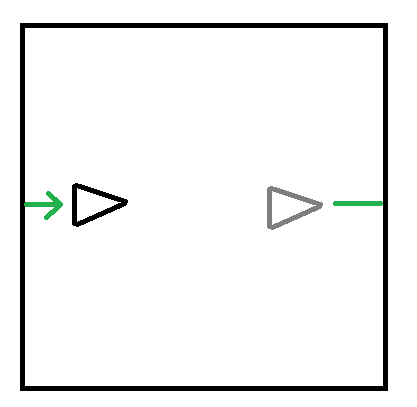
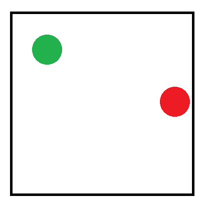


 , instead of
  .
.
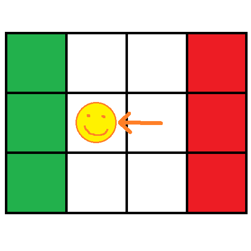
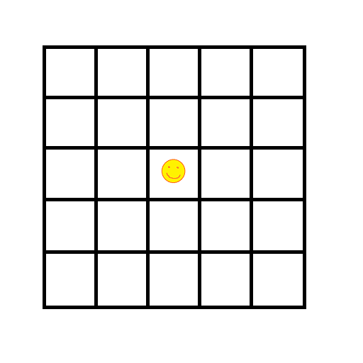
 .
.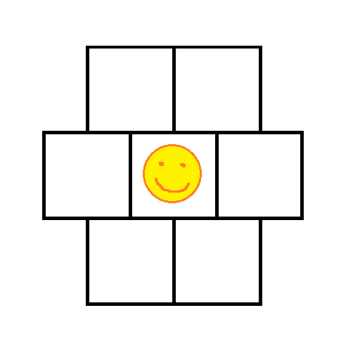
 cells in memory.
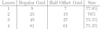
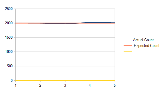
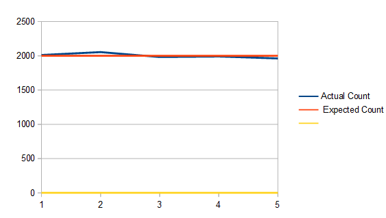
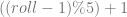 . This works because there is no remainder for 20 % 5. If there was a remainder it would bias the rolls towards the numbers <= the remainder, making them more likely to come up than the other numbers.
 .
. where x is in [0,1) and I'm using a box that goes from (0,0) to (1,2) to get 100,000 samples.
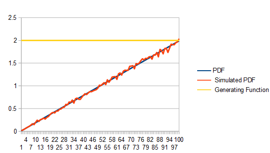
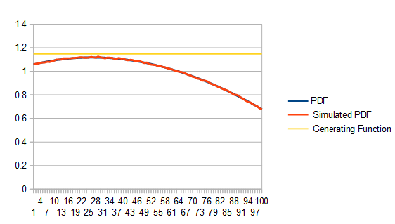


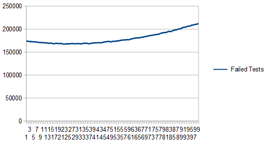


 , you can use any PDF
  to do so, so long as you multiply
  so that
 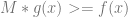 for all values of x. In other words: scale up g so that it’s always bigger than f.
 . We’ll use an
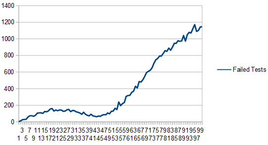


 where
where ![x \in [0,1]](https://s0.wp.com/latex.php?latex=x+%5Cin+%5B0%2C1%5D&bg=ffffff&fg=666666&s=0&c=20201002) . The graph looks like this:
. The graph looks like this:
 where
where 


 which looks like this:
 and looks like this:


 . The area under that curve where x is in [0,1) is 1.0 and it’s non negative everywhere in that range too, so it’s a valid PDF.
 for the CDF. Then we invert the CDF:
![y=x^3 \Leftarrow \text{CDF}\\ x=y^3 \Leftarrow \text{Flip x and y}\\ y=\sqrt[3]{x} \Leftarrow \text{Solve for y again}](https://s0.wp.com/latex.php?latex=y%3Dx%5E3+%5CLeftarrow+%5Ctext%7BCDF%7D%5C%5C+x%3Dy%5E3+%5CLeftarrow+%5Ctext%7BFlip+x+and+y%7D%5C%5C+y%3D%5Csqrt%5B3%5D%7Bx%7D+%5CLeftarrow+%5Ctext%7BSolve+for+y+again%7D&bg=ffffff&fg=666666&s=0&c=20201002)


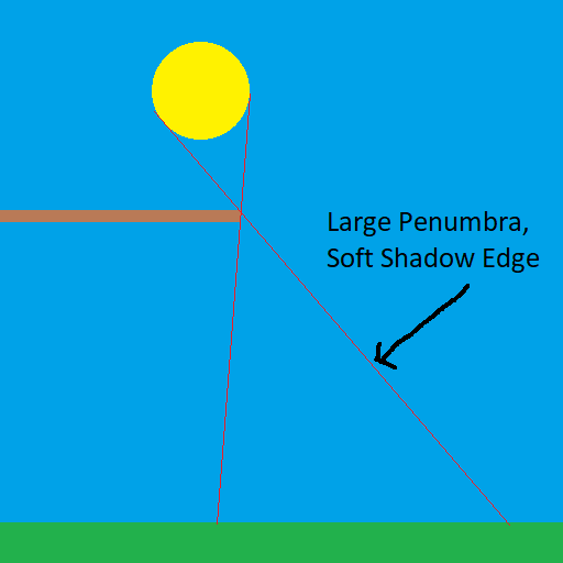
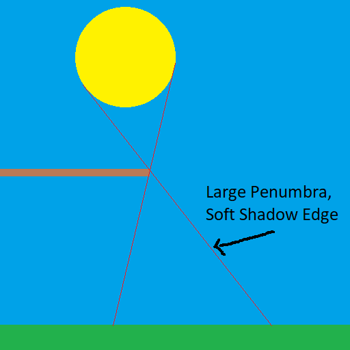
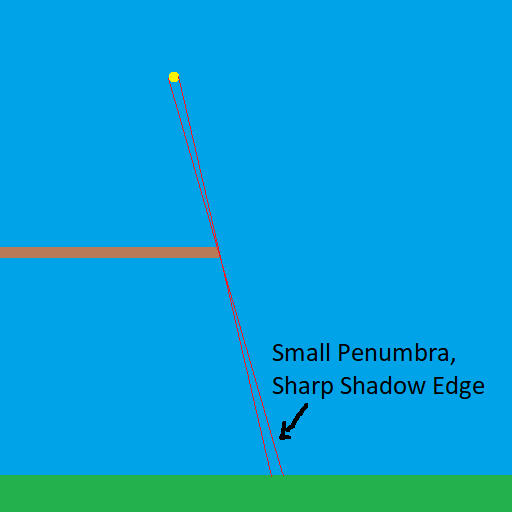
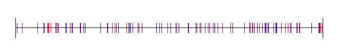
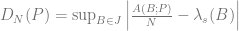
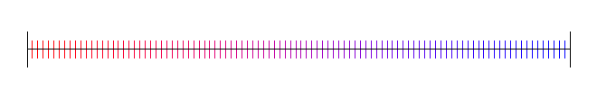

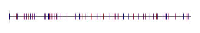


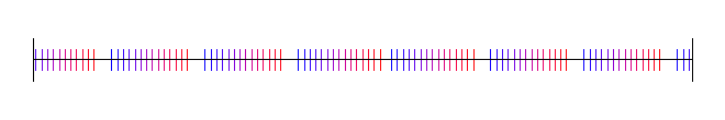
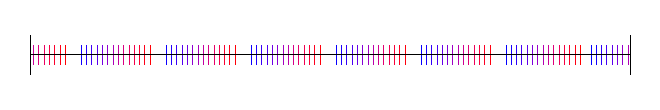
 ,
,  ,
,  , etc (where B is the base), you instead treat them as
  ,
,  ,
,  and so on. In other words, you multiply each digit by a fraction and add up the results.
 , so we can see that 110 is in fact 6 in binary.
 .
. .
.
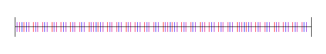

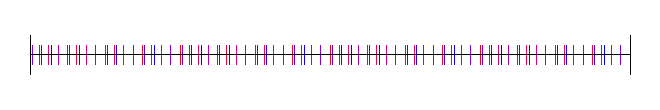
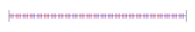

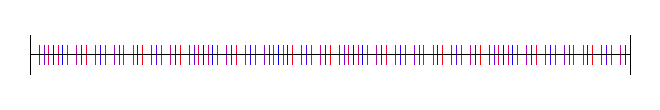


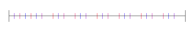
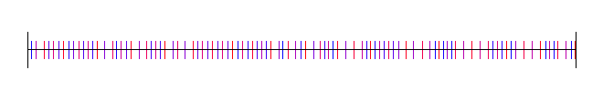

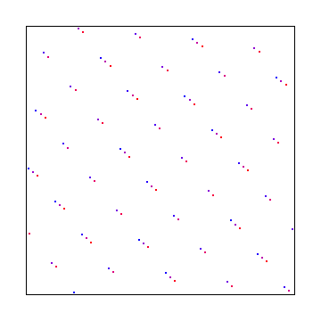
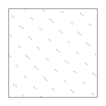
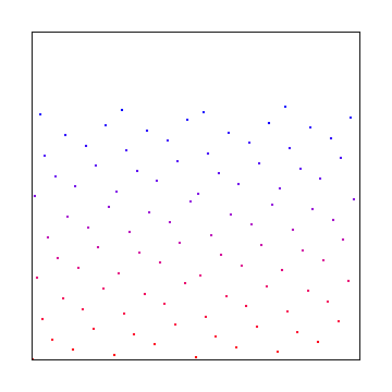
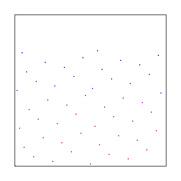
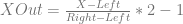
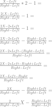


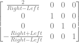
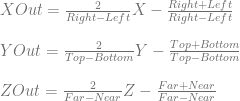


 to
to  which has the same effect, and would give you something like this:
