This post explains how Russian Roulette can be viewed as rejection sampling a PDF to do importance sampling.

The explanation sticks to simple 1D functions and has some ~500 lines of c++ to accompany it that made the data for the explanations.

The code is at: https://github.com/Atrix256/RussianRoulette1D

Background Topics

Here are some quick definitions and links to more info.

Monte Carlo Integration – Using random samples of a function to find the area under the curve if you graphed it. Aka using random numbers to integrate a function numerically.

Importance Sampling – Using random numbers in Monte Carlo integration where the probabilities of numbers drawn aren’t the same for each number. As the graph of the probabilities looks more similar to the graph of the function being sampled, Monte Carlo integration gets closer to the right answer a lot more quickly. At the extreme, it only takes one sample to get the exact answer!

PDF – Probability density function. This is a function that describes how probable different numbers are for being generated. It integrates to 1, but might have values that go above one. The area under the curve between 2 values is the percent chance probability of a random number falling between those two values.

Uniform Distribution – Random numbers (A PDF) where all possible values are equally likely. If you made a histogram of the numbers generated from this distribution, it would be flat, if you generated an infinite number of values.

Rejection Sampling – If you know the shape of a PDF you would like to draw random numbers from, but you aren’t sure how to actually generate random numbers following that PDF, rejection sampling is one way to do that.

Russian Roulette – If you have something like an infinitely recursive (or iterative) integral, like you find with the rendering equation, Russian Roulette is a way to stop the infinite process early while still getting the correct answer. It stops early without adding bias. More generally it lets you skip doing some of the work you have to do, without adding bias.

Here are the links:

Monte Carlo Integration Explanation in 1D

Generating Random Numbers From a Specific Distribution With Rejection Sampling

Russian Roulette and Splitting (PBRT book chapter 13.7)

You’ll also see the code for this post doing a “lerp” to average sample points. If you want more info about that, check this out:

Incremental Averaging

Integrating y=x^2 from 0 to 1

Let’s look at a couple different ways to integrate a function numerically, to get a sense of things.

We’re going to integrate y=x^2 from 0 to 1 three different ways. First we’ll use regular Monte Carlo with a uniform distribution, second we’ll importance sample it using rejection sampling, and thirdly, we’ll use Russian roulette which as you’ll see is also importance sampling using rejection sampling.

Simple Monte Carlo integration works like this:

1. Take N random samples of a function between A and B
2. Sum them up and divide by N to get the average height of the function between A and B
3. Multiply by B-A to get the area under the curve

Doing that with the accompanying code, after 1000 samples the value it comes up with is 0.298374. The actual value is 1/3 or 0.33333… so it got fairly close. Check out the “// monte carlo” section in the code inside of TestFlat().

We’ll do the same steps again but this time do importance sampling with rejection sampling.

Since we know y=x^2 is 0 when x is 0 and 1 where x is 1, we can use rejection sampling to make a probability density function that is similar.

Whenever we generate a random number “x” between 0 and 1 to use in the function, we’ll say there is an “x” percent chance that we keep that number, otherwise we throw it away and generate a new random number. Another way of saying this is that there is a 1-x percent chance that we are going to throw it away and generate a new random number.

That probability of keeping numbers looks like the function y=x when you do this. y=x isn’t a proper PDF though because the area under the curve is 0.5, not 1, so you need to multiply it by 2 to make it a proper PDF. This doesn’t actually change the probabilities, this is just making a “proper PDF” that describes the probabilities. So, the PDF for these random numbers is y=2x.

We have to change how we use these random numbers too though. After we calculate our y value by plugging x into y=x*x, we need to divide it by the PDF value for x before we add them to the sum (the sum which we later divide by N to get the average). You just plug x into the PDF function y=2x to get the PDF value. We divide by the PDF because what this does is make it so numbers that come up more often weigh less into the final average. For instance, if one number came up twice as often than another in your random numbers, you should make it count for half as much to the final average, to make things equal like they are in plain vanilla Monte Carlo.

When we do this with 1000 samples, we get a value of 0.334112 (Monte Carlo was 0.298374). You might find it interesting that we had to generate 2052 potential x values for the 1000 we actually used. 1052 were thrown away.

Next up we are going to do Russian Roulette. How this works is we are going to have a probability where we just aren’t going to take a sample AT ALL. We are going to modify the first step of the Monte Carlo algorithm:

1. Take N random samples of a function between A and B. There is some percent chance “p” we won’t actually do a sample, but will just use a value of 0. If we do take a sample, we are going to divide the value we got by 1-p which will make it a larger value to make up for the times we didn’t take a sample.
2. Sum them up and divide by N to get the average height of the function between A and B
3. Multiply by B-A to get the area under the curve

If we do that with a probability of 1-x of killing a sample (aka an “x” percent probability of using a sample. Is this sounding familiar?), and do 1000 attempts, we get a value of 0.327171. We didn’t do as well as we did with importance sampling using rejection sampling, but that used a full 1000 samples, while this method only ended up using 746 samples actual samples.

So:

In the rejection sampling algorithm, we used x as the percent probability to determine whether we actually plug that x into the function, or a 1-x percent probability to generate a different x value. We loop until success.

In the Russian roulette algorithm, we used 1-x as the percent probability to use 0 instead of taking a sample, or x as the probability to take a sample and divide it by (1-x) to make it larger to make up for samples we killed.

Does those sound pretty similar to you?

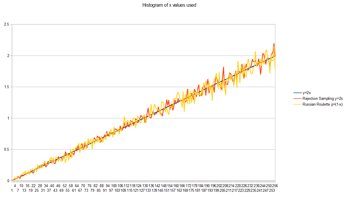
As further evidence, here’s the histogram of x values generated by each of those algorithms, along with a graph of the PDF y=2x, modifying the code to take 100k samples instead of 1000, to reduce the random noise in the graph (make it converge more). This shows that they are generating random numbers from the same PDF, which is y=2x.

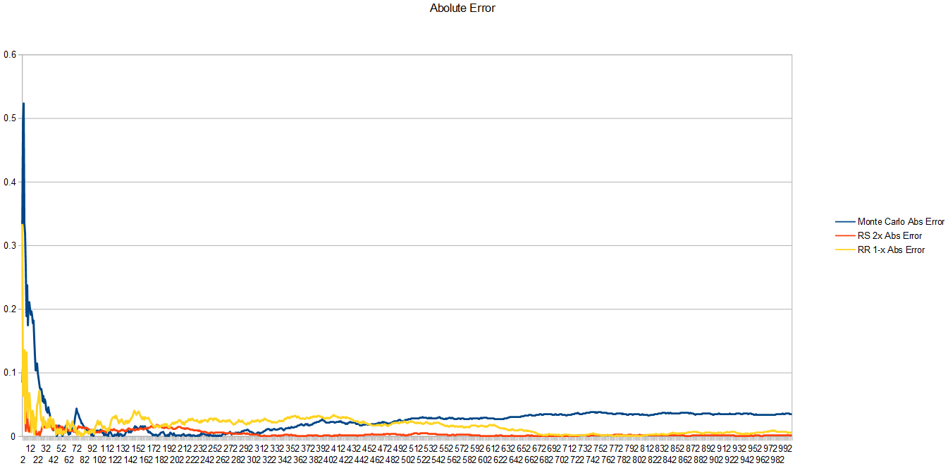
Here is the absolute error of each technique for each sample. Rejection sampling a PDF of y=2x is showing lowest error, followed by Russian Roulette with a probability of 1-x to kill a sample, and lastly in the rear comes vanilla Monte Carlo. It’s important to remember that rejection sampling and monte carlo are taking new samples each time you take a step forward on the x axis, but for russian roulette, it’s sometimes not taking a sample and just using a value of 0 instead.

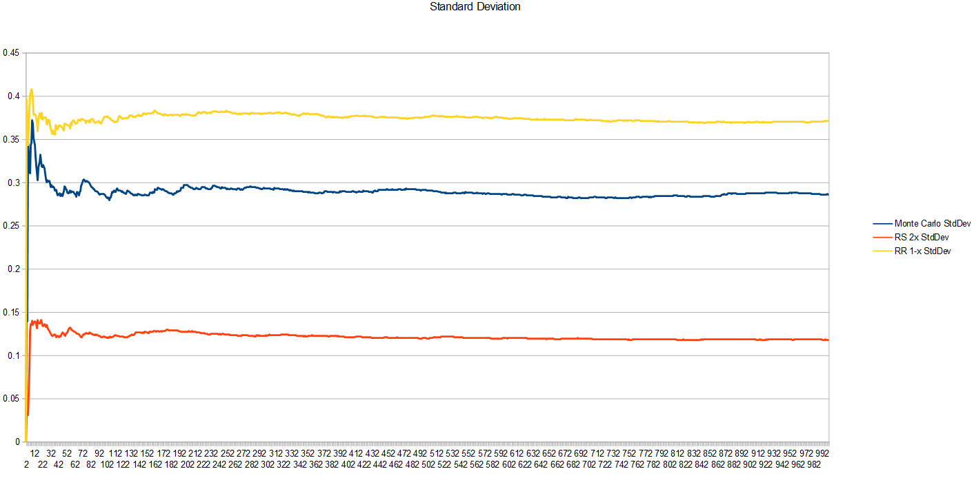
Looking at the standard deviation, the square root of variance, this tells us how erratic the samples are.

Unfortunately, the worst variance comes from the Russian Roulette algorithm. I don’t have a good sense of why this is or how it can have worse variance than Monte Carlo but come up with a better result. Mathematically, I know the reason is due to the zeroes used when a sample is killed, but intuitively, I don’t grok how this can be true or what it means exactly to be better converged, but have worse variance. Something to chew on I guess (or feel free to educate me if you know!)

Why Does Russian Roulette Boost Values?

Ok so let’s take a quick break to get some intuition for why Russian roulette boosts values up when they survive the random killing.

Let’s say we have a function y=1, so it’s just a function that is 1 everywhere.

If we wanted to integrate that from 0 to 1 with Monte Carlo using four uniform random samples, we’d get four 1s, sum them up to get 4, divide by the number of samples (4) and get our result of 1.

That’s the right answer: a function that has a y value of 1 everywhere, for x being between 0 and 1 is a square of length 1 on both the x and y axis. That square has an area of 1.

If we wanted to use Russian roulette here with a 25% chance to kill a sample, we could assume that one of our four samples was killed. That means we get 3 samples each getting a value of 1, and the sample we killed has a value of 0.

If we sum the samples we’d get 3. If we divide them by the number of samples taken, we’d get 3/4 or 0.75.

This is the incorrect answer!

Since we know we are going to kill one out of every four samples, what we could do is boost every survivor to make up for the samples we killed.

The algorithm says we divide by 1 minus the probability, which is in this case 0.75 or 3/4.

Dividing by 3/4 is the same as multiplying by 4/3.

So, going back to our samples we have four samples. Three of them were 1, multiplied by 4/3 to get 4/3. The last sample was killed so is 0.

Summing these samples up, we get 12/3 which reduces to 4.

Dividing that sum by the total number of samples (4) we get 1.

That is the RIGHT answer.

Russian roulette boosts the survivors to make up for the missing information of the samples that were killed.

Sure, it’s random, and the boost amount may not actually match the number of samples actually killed, but given enough samples it’ll be true, or close enough to true.

Bonus: use blue noise or low discrepancy sequences to make this be more true for smaller sample counts.

Iterative / Recursive Functions

You might be saying to yourself that this example is stupid, because nobody uses Russian Roulette this way, and you may in fact be doubting that it is Russian Roulette because it’s used in such a foreign setting.

The usual place you see it used if you are a graphics person is in terminating a ray while it’s bouncing around a scene so that you can kill it early without bias, when the ray isn’t likely to be contributing much value to the result if it continues.

Well, same thing applies. Using it in this setting just lets you say “ah screw it, i’m stopping here” with some probability. The rest of the time, the values you DO get are boosted up to make up for the slackers who quit early.

The only real difference is that because it’s recursive, each survival grows the weight of not only the current iteration but all future iterations too – this is because the current iteration relies also on the future iterations.

Let’s quickly see some data for a recursive/iterative function:

1. calculate y = f(x) = sin(x*pi/2)
2. Divide x by 2 and do it again
3. Do this 1000 times
4. The sum of the above is the result

We are going to integrate that from 0 to 1, meaning we are going to take random numbers between 0 and 1, plug them into the above, and the average will be the area under the curve.

After doing this 10,000 times…

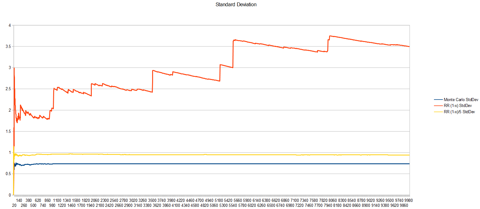
Monte Carlo gives us a value of 1.403612 with a standard deviation of 0.733499.

Since the basic function sin(x*pi/2) is 0 when x is 0 and 1 when x is 1, i used the same probabilities for Russian Roulette as before. That gave me a value of 1.285901, with a standard deviation of 3.493362. Instead of doing a full 1000 loops through the function though, for those 10000, it did 0 loops at minimum, 5 at max, and 0.71 on average. That is quite a savings on iteration count.

To be honest, i’m not sure what the right answer to this function is, so i can’t say how correct these answers are (A less lazy person would run Monte Carlo with a very large number of samples). They are pretty close to each other though which makes me think they must be in the ballpark. If that’s true, they have fairly similar error (at least in a spherical cow sense), but one did 1000 iterations, while the other did 0 or 1 on average, and 5 maximum. That is pretty cool! Admittedly the variance got worse again though.

Using a different probability for Russian Roulette, where the PDF more closely matched what the actual shape of the function was (the iterated function, not just a single incarnation of it?) would get you a better answer quicker. i didn’t really experiment with that very much.

I did think that 0 to 1 iterations on average was pretty low though, so instead of making the probability be 1-x to kill a sample, i tried making it (1-x)/5. That way, the probability shape is still the same, but samples are less likely to be killed, so they should survive more iterations.

That did in fact work!

After doing that 10,000 times, Russian Roulette gave a value of 1.378251 with a standard deviation of 0.939193. The minimum number of iterations is still zero, but the maximum went up to 45, and the average went up to 4.89. We got to keep the shape of our PDF, but got deeper through the iterations. So, we are sort of importance sampling on 2 axes – fun 😛

The value changed and I’m unsure if it’s for better or worse, but it got closer to the plain Monte Carlo answer, which is a good sign. The variance also got better which is neat, but is still worse than the Monte Carlo variance.

Here’s a graph of the value of the functions as the number of samples grow:

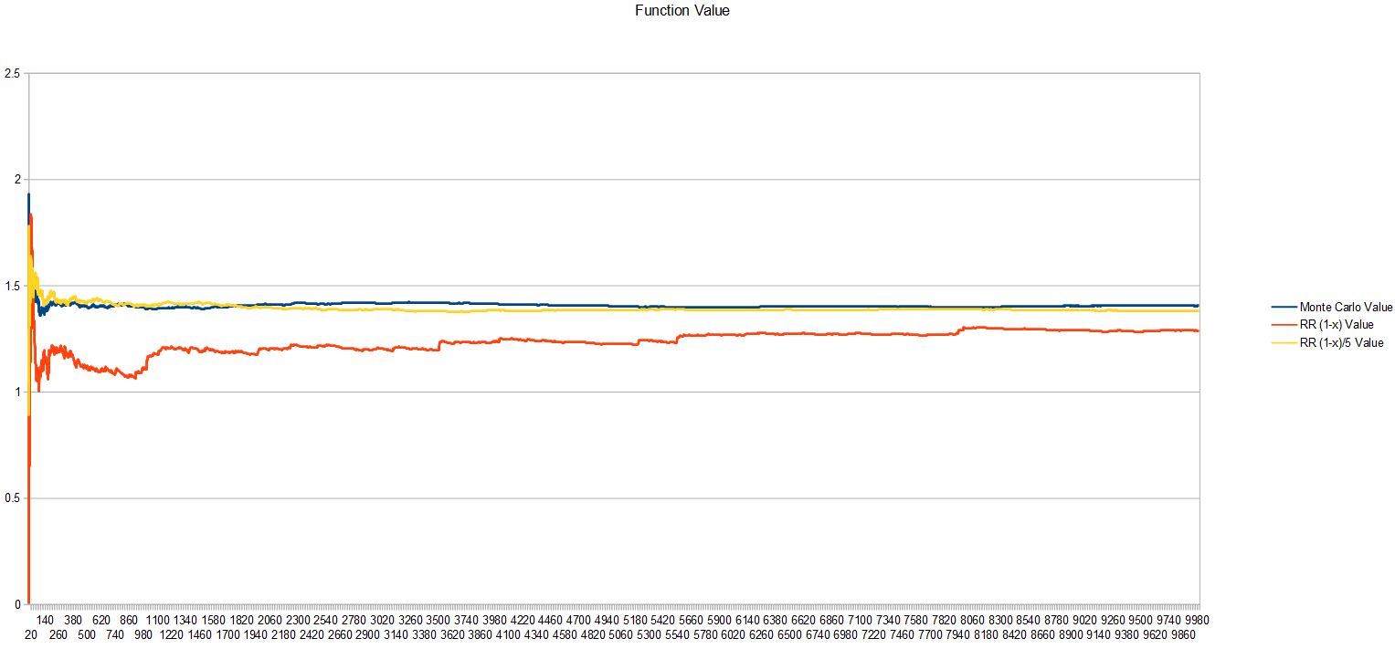
Here’s a graph of the standard deviation. The probability 1-x has really bad variance, while dividing it by 5 has much better variance.

Closing

So hopefully you now can see a link between Russian Roulette and importance sampling using rejection sampling.

What I found neat about this perspective is that instead of Russian Roulette being some “one off” technique, I can merge it mentally with rejection sampling and importance sampling, and free up some brain space.

I also like this “off brand” of Russian Roulette.

Basically, rejection sampling is a “no go” for real time graphics in general, like for use in a shader. The reason for this is that rejection sampling takes an unknown number of iterations each time to generate a single valid sample.

If you instead use Russian Roulette, it’s a fixed upper bound amount of work, but you will get some randomly less number of samples of your data.

Another way to put it is that when generating numbers from a PDF…

• Rejection sampling requires an unknown sized loop to generate a fixed number of samples
• Russian Roulette has a fixed loop to generate an unknown number of samples

Engineering is all about trade offs, so having this trade off is pretty handy IMO.

Let’s do a quick, simple recap on Rejection Sampling vs Russian Roulette for integrating a y=f(x) function using a specific PDF.

I’m defining a function A(x) which is the probability of accepting a value “x” chosen. The function A is just a scaled version of the PDF such that all values in the PDF are <= 1. This function gives you the probability of keeping a value "x" after randomly selecting it – for both rejection sampling, and russian roulette.

Rejection Sampling

1. Draw a number x from a uniform distribution between a and b.
2. Roll a random number from 0 to 1. If that number is greater than A(x), go to 1.
3. calculate y=f(x)/pdf(x) to get a sample
4. The result of the integral is the average y value, multiplied by (b-a)

The count of random numbers you had to generate is dynamic, to get a fixed number of samples.

The number of random x’s generated is >= the number of samples you got out.

The count on the left changes.

Russian Roulette

1. Draw a number x from a uniform distribution between a and b.
2. Roll a random number from 0 to 1. If that number is greater than A(x), y=0
3. Else, y=f(x)/A(x)
4. The result of the integral is the average y value, multiplied by (b-a)

The count of random samples you had to generate is fixed, to get a dynamic number of samples.

The number of random x’s generated is still >= the number of samples you got out.

The count on the right changes.

Last thing: I could be wrong, but i believe that Rejection Sampling is a “Las Vegas” algorithm, while Russian Roulette is a “Monte Carlo” algorithm.

https://en.wikipedia.org/wiki/Las_Vegas_algorithm#Relation_to_Monte_Carlo_algorithms

Assuming i’m correct in my understanding there, Monte Carlo algorithms are preferred in real time graphics, games, and other real time situations. The ability to have knowledge or control over how long something will take to execute is in general way more important than the quality of the result you get. In modern times of temporal accumulation, this is even more true, since poor data every now and then can be soaked up by the temporal accumulation, to an extent.

And in those situations, you can do even better by using random or quasi random sequences which have better properties over both space and time, to help ensure that you get better results over smaller regions of space, and over shorter periods of time.