In 2017 I wrote a couple blog posts looking at animating noise for integration over time:
https://blog.demofox.org/2017/10/31/animating-noise-for-integration-over-time/
https://blog.demofox.org/2017/11/03/animating-noise-for-integration-over-time-2-uniform-over-time/

Recently we put out some research work I did with some other people at NVIDIA that is essentially the part three:
https://github.com/NVIDIAGameWorks/SpatiotemporalBlueNoiseSDK

This blog post is a follow up blog post to one I wrote in 2018 that showed some subtle but important differences in blue noise textures:
https://blog.demofox.org/2018/08/12/not-all-blue-noise-is-created-equal/

In this blog post we look at some different types of blue noise in frequency space, including the new spatiotemporal blue noise types.

The source images and python processing script that generated the images in this post can be found at: https://github.com/Atrix256/BNDFTInvestigations

Some Memes

First, some spatiotemporal blue noise memes 🙂

How Do You Analyze Frequencies of Vector Valued Blue Noise Textures?

The “Blue-noise dithered sampling” paper (https://www.arnoldrenderer.com/research/dither_abstract.pdf) was the first paper to make vector valued blue noise textures. In that paper, they did frequency analysis by DFTing each axis (color channel) separately and showing the results in the respective color channels.

That’s what we did as well in our spatiotemporal blue noise work, but it doesn’t tell the whole story. What this method tells you is that the X axis is blue noise, the Y axis is blue noise and the Z axis is blue noise, but it doesn’t tell you that the 3D vector itself is blue noise. There is in fact a whole paper regarding the difference between vectors as a whole being blue, or their individual components being blue, and how some insights there can lead to better image quality and convergence! (Projective Blue Noise: http://resources.mpi-inf.mpg.de/ProjectiveBlueNoise/ProjectiveBlueNoise.pdf).

Is there a way to do a Fourier transform of a texture full of vectors?

Spherical harmonics comes to mind, but I couldn’t reason out how you could use it for that purpose. You could use SH to fit all the vectors in a texture but you could shuffle the pixels in the texture and get the same results so that doesn’t seem right. It seems like you’d need to start with getting SH to be able to fit a 1D stream of (time series) vectors, and then extend it to 2D.

There is also apparently a way to do a Fourier transform in Clifford analysis that seems promising, but it’s above my understanding so am not sure how it works, or if it really even does work for this case (https://en.wikipedia.org/wiki/Clifford_analysis#The_Fourier_transform).

Another method was suggested to me on twitter and I’ve lost the tweet unfortunately and can’t remember who sent it to me. If it was you, or you remember who it was please let me know so I can say thank you and give credit! The idea was to take the DFT of each component (which results in a complex number per pixel, per color channel), get the magnitude of each pixel in each component (which results in a real number per pixel, per color channel) and then treat that as an N dimensional vector that you take the magnitude of for the final result. This seems to work well but I can’t explain why it works, so am not certain about it.

In the image below, the top row is a blue noise texture where the red and green channels each have independently generated blue noise. The “DFT Single” column shows that when looking at the DFT of each channel separately, it shows blue noise – a dark hole in the low frequencies in the middle, and randomized higher frequencies. When looking at the DFT combined as described in the last paragraph, it shoes a pinkish noise type frequency content though – strong low frequencies, and then white noise added on top. In contrast, the 2nd row noise was made with the “Blue-noise dithered sampling” paper’s method of making a true vec2 valued blue noise texture. The “DFT Single” row shows blue noise again, and the “Combined” column shows blue noise as well. This is what we’d expect because the scalar RG row makes the X and Y values of the vectors independently, and doesn’t care about the frequencies of the vectors made form combining them. The Vec2 RG row is made considering the combined vectors, on the other hand. You can see similar results for the Scalar RGB and Vec3 RGB rows. All textures are 64×64, 8 bit per color channel pngs.

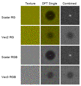
The blue noise is much less pronounced in the true vector valued blue noise textures. Does this mean there is higher quality vector valued blue noise waiting to be found? I’m not sure, but I do think so. In our spatiotemporal blue noise work, we found that blue noise made with the void and cluster algorithm were higher quality than those made with the “blue-noise dithered sampling” method when generating scalar noise with each.

2D DFTs

Next up let’s look at 2D slices and DFTs of those 2D slices of different types of blue noise textures. “Blue 2D” is 64 different 2D blue noise textures generated, each being 64×64. “Blue 2Dx1D” is spatiotemporal blue noise which is 64x64x64 (not included in the repo for this blog post, and generated with the code here: https://github.com/NVIDIAGameWorks/SpatiotemporalBlueNoiseSDK). “Blue3D” is 3D blue noise which is 64x64x64. We’ll look at both XY slices and XZ slices.

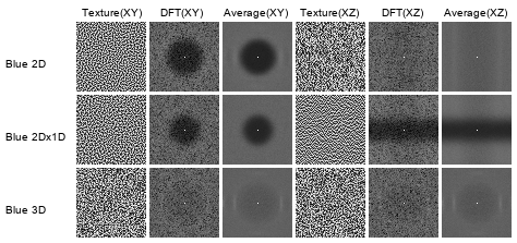
One interesting thing to see is that 3D blue noise looks the same when sliced on XY or on XZ while the other two are very different. Another is that the spatiotemporal blue noise has a lower cutoff frequency than the 2D blue noise. Maybe adjusting energy sigmas on time vs space could change that. Also, of course, 2D blue noise is white noise on the Z axis while the spatiotemporal blue noise has attenuated low frequencies on the Z axis.

3D DFT – Blue 2D

When we take a 3D DFT of a 64x64x64 image, we get frequency magnitudes that are also 64x64x64. It’s hard to visualize that so I’ll show slices of the 3D DFT – first the XY aligned slices, then the XZ aligned slices to get a different view of the same data.

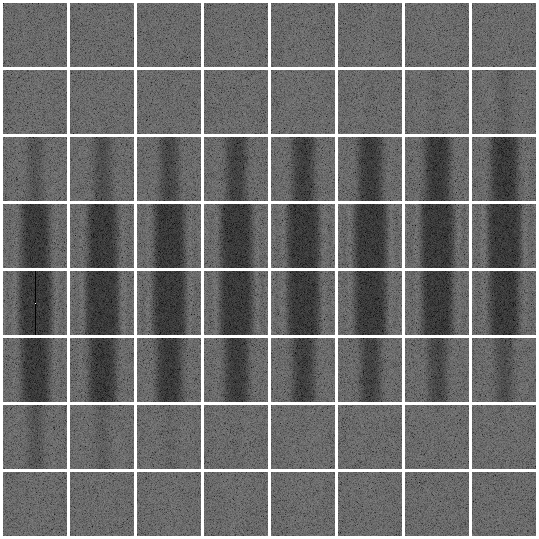
First is 2D blue noise – 64 different 2D blue noise textures that are each 64×64. Here are the XY slices with slice 0 in the upper left, slice 1 to the right of it, and slice 63 in the lower right.

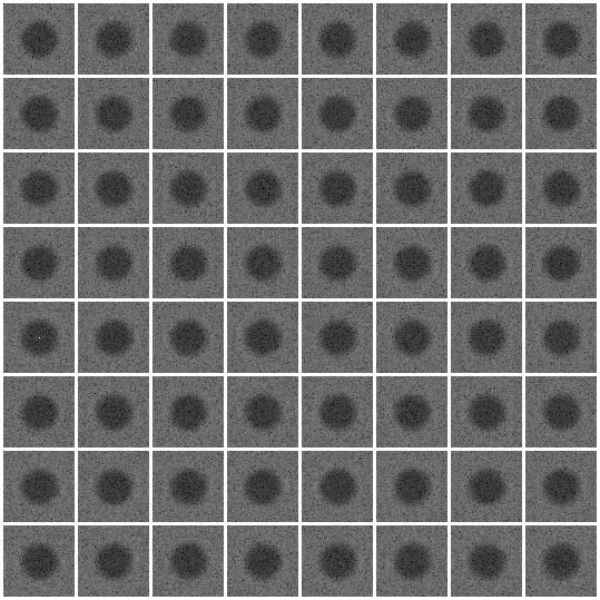
Here are the XZ slices which just show cross sections of the cylinder we were looking at in the XY slices. At slice 32, there is a vertical black line with a white dot in it. That white dot is DC, but I’m not sure why that black line is there.

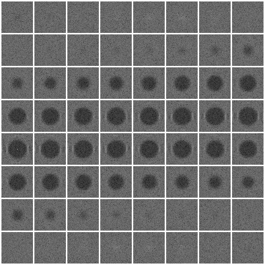
3D DFT – Blue 2Dx1D

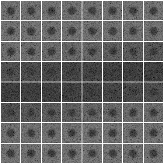
Next is the 2Dx1D blue noise, or spatiotemporal blue noise. First are the XY slices:

Then the XZ slices:

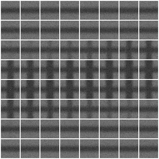
This spatiotemporal blue noise looks the same as the 2D blue noise we saw last, but with a darkening of all frequencies near where Z is zero. This is what we expect and hoped for: it’s 2D blue noise but also has attenuated low frequencies on the z axis (time).

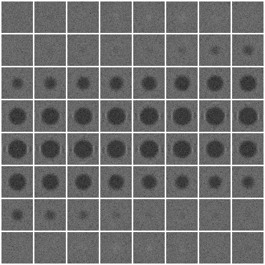
3D DFT – Blue 3D

Here are the XY and then XZ slices of the 3D DFT of 64x64x64 3D blue noise. The 3D DFT is a darkened sphere surrounded by white noise, which is what we see in the slices as well, with a circle that grows and shrinks, like if you took slices of a sphere.