Using Wang Tiles to Simulate Turing Machines

Wang tiles were invented by Hao Wang in 1961 for mathematical reasons, but they find great use in games for making tile based art which gives results that don’t look tiled – both with 2d tiled textures, as well as 3d tiled models.

Apparently Wang tiles are also able to execute Turing machines, and so are thus Turing complete – meaning they can execute any program.

That is a pretty amazing and perplexing statement, so this post explores that a bit.

Wang Tiles Overview

Wang tiles are rectangular tiles where each edge will only fit with other specific edges, but that for any specific edge, there is more than one possible tile that can fit with that edge. By fit with that edge, I mean they are seamless when put together, without any visual artifacts to hint at there actually being a seam between the tiles.

This is useful for graphics because this lets you have seamless tiled graphics, but the specific configuration of how the tiles are placed can be completely randomized, so long as their edges are all compatible. The result is tiled graphics that doesn’t look at all tiled, due to visible patterns being much less noticeable than with traditional tiled graphics.

For graphical examples, a little more info and some links to some shadertoys check this out: Wang Tiling

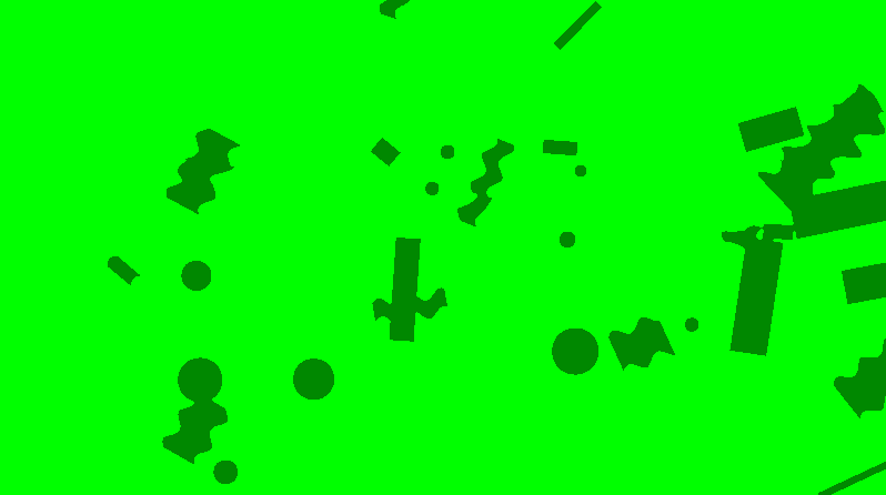
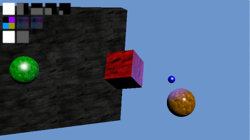
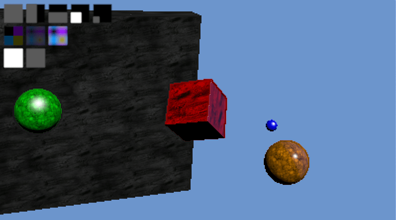
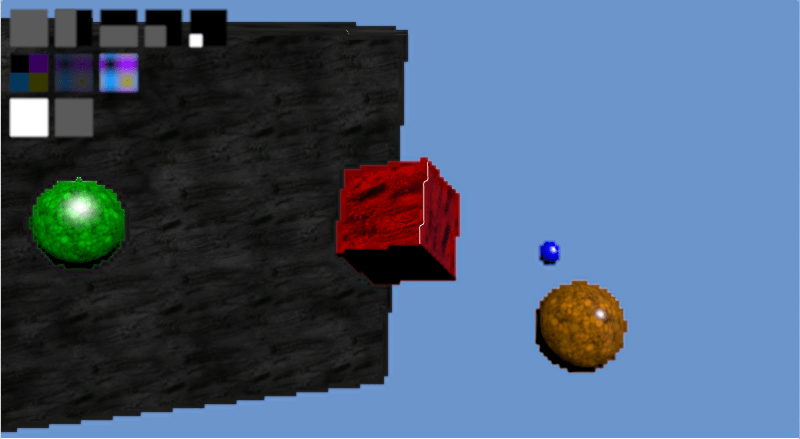
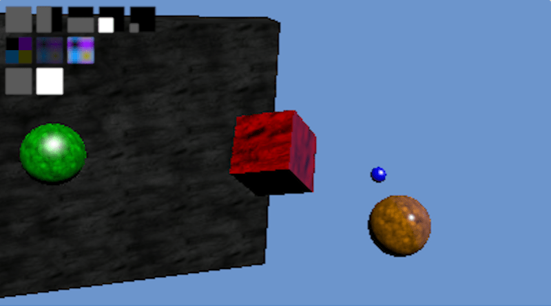
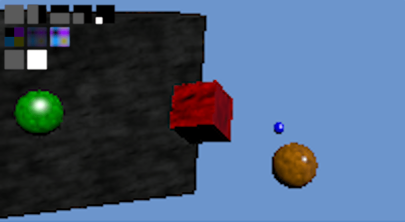
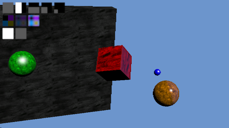
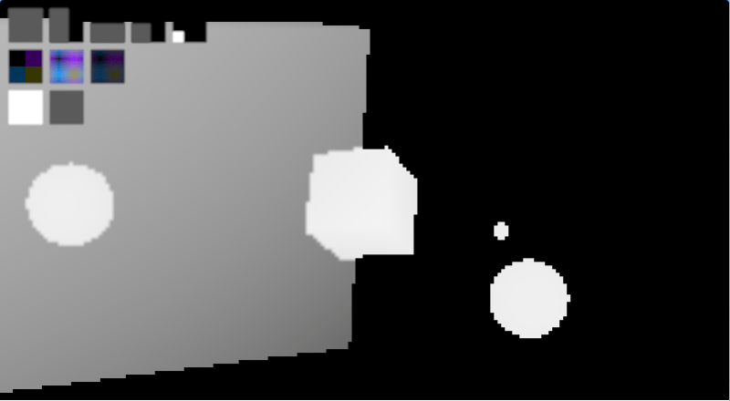
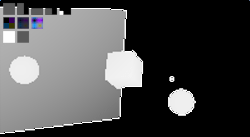
Here is an example I made. The graphics are programmer art but hopefully you get the idea. This was made with 16 tiles, where there were two different edge types per edge.

Turing Machine Overview

Turing machines were invented in 1936 by Alan Turing as a generic computing machine that was proven to be able to execute any algorithm.

The turing machine is made up of a few main components: the memory tape, the read/write head, and the state machine.

The memory tape is infinitely long, so has infinite storage, and is initialized to all zeroes to start out.

The read/write head starts at a position on the tape, and can read or write values, and also move left or right on the tape.

The state machine controls the read/write head.

The state machine knows what state it is in and has rules about what to do in each state when it reads a value from the tape.

For instance, in state A, if a 0 is read from the tape, the rule may be to write a 1 to the current position on the tape, move the read/write head to the right, and go to state B. State B may have completely different logic, and could either transition back to state A, state in state B, or move to another state entirely.

Using simple state transition logic like that, any computer algorithm can be performed.

In a Turing machine there can also be a “Halt State” which means the program is finished executing and the answer it was trying to calculate has been calculated.

Looking at some programs, you can easily see that they will halt eventually, or that they will be an infinite loop and never halt. Some programs in-between are complex and can’t very easily be determined if they will ever halt or not. Turing proved that there is no general solution to whether a Turing machine (aka any computer program) will halt or not, and this is called the Halting Problem. In general, the only way to know if a program will halt or not is to wait and see. So, effectively the answers to whether a program in general will halt or not are “yes” and “not yet” – although for many specific programs you can in fact see that they will halt eventually if you were to run them.

Wang Tile Computation

It turns out that Wang tiles can simulate a Turing machine, and so are “Turing complete” meaning that they too can perform any computer algorithm.

To make this happen, we’ll make a column of tiles that represent the state of the Turing machine at a specific point in time, starting with time 0 at the left most column. We’ll place tiles in the column to the right making sure all edge rules are respected, and then do the column to the right of that one etc until the program halts (or forever if it doesn’t halt). If we set up our set of tiles correctly, the act of satisfying the edge rules as we place our tiles is enough to execute the Turing machine.

Let’s walk through a simple example where we have the following state machine logic rules:

  1. When in state A, if a 0 is read, we will write a 1, move the read/write head down and move to state B.
  2. When in state A, if a 1 is read, we will halt (enter the halt state).
  3. When in state B, if a 0 is read, we will write a 1, move the read/write head up and move to state A.
  4. When in state B, if a 1 is read, we will halt (enter the halt state).

Tape Memory Storage

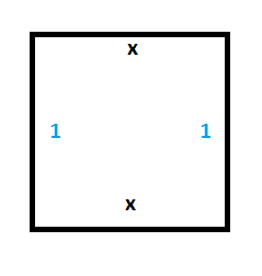
The first thing we need is persistent storage of memory for the tape. For this, we’ll need the following two tiles:

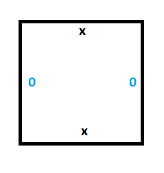
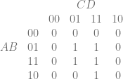
To see this working, we can set up a section of tape with some values (make a column of wang tiles), and we can see that the only valid wang tiles to place next to the starting column are tiles which propogate the 0 and the 1 values forward in time without modifying them.

In the diagram below, we initialize the tape to 0101 in the left most column (time 0). By only placing down tiles with compatible edges you can see that our memory values persist forever. Our memory storage is implemented, huzzah!

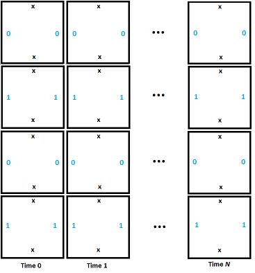
We’ll start our example with all memory initialized to 0, but the above shows that we can have persistent memory.

Read/Write Head State Machine

The read/write head of the Turing machine is represented as part of the edge information. In this way, besides an edge storing the 0 or 1, if that is where the read/write head is, it also stores the state of the state machine.

Our example uses two states (besides the halt state): A and B. If a 1 is read in while being in either state A or B, the program halts.

To handle that, we need the tiles below:

Now that we have the rules for entering the halt state done (rule #2 and rule #4), we have to figure out how to implement the rules that control switching from one state to another (rule #1 and rule #3).

Moving the Read/Write Head

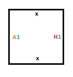
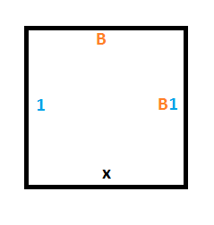
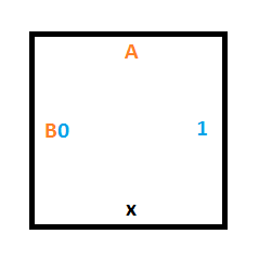
Rule #1 says that if we are in state A and read a 0, we should write a 1, move the read/write head down and move to state B.

We’ll need this tile to cause reading a 0 in state A to write a 1 as output, and to tell the tile below to move to state B.

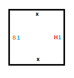
The tile below that one could either be a 0 or a 1, and without knowing which, we want it to keep it’s value but accept the read/write head and be in state B. To do that we need two tiles, one for if there is a 0 on the tape at that position, and another for if there is a 1 on the tape.

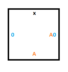
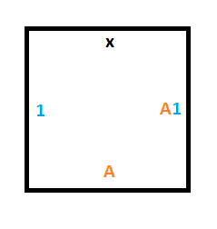
Rule #3 says that if we are in state B and read a 0, we should write a 1, move the read/write head up and move to state A.

To do that, we’ll need a similar construction as for rule #1 but we are moving up instead of down. These 3 tiles will give us what we need:

Starting Column Tiles

We are going to treat the boundaries of our simulation area as if they have edges of “x”.

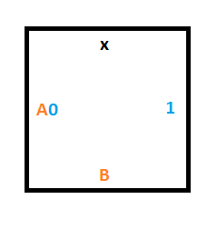
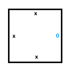
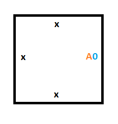
This means that to make our starting column (the Turing machine at time 0), we are going to need 2 special tiles. One tile will be for storing a 0 on the tape, which is what the tape is initialized to, and the other tile will be for storing the position of the read/write head in state A, which is our starting state.

Here are those two tiles:
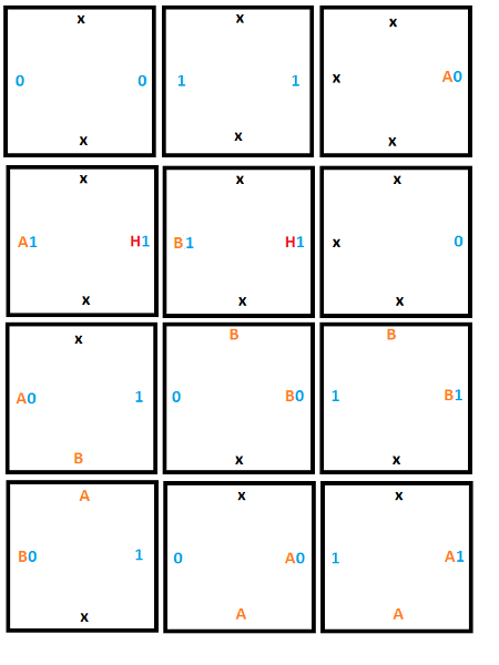
Final Tileset

Here’s the full set of 12 tiles that we are going to use:

Full Simulation

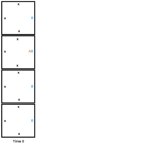
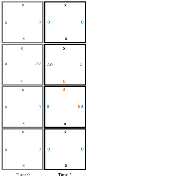
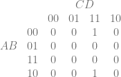
Here is the initial setup at time 0 for our Turing machine. Note that this is one possible starting state, but this is the starting state we are choosing. We are not leaving it up to chance where the read/write head starts, or if it is even present at all. If we only followed edge rules we may get 4 read/write heads or 0, or anything in between.

From here, to build the second column, we start from the top and work towards the bottom, choosing the tile that fits the constraints of the edge it touches. In this first step, the head reads a 0, writes a 1, moves down, and moves to state B.

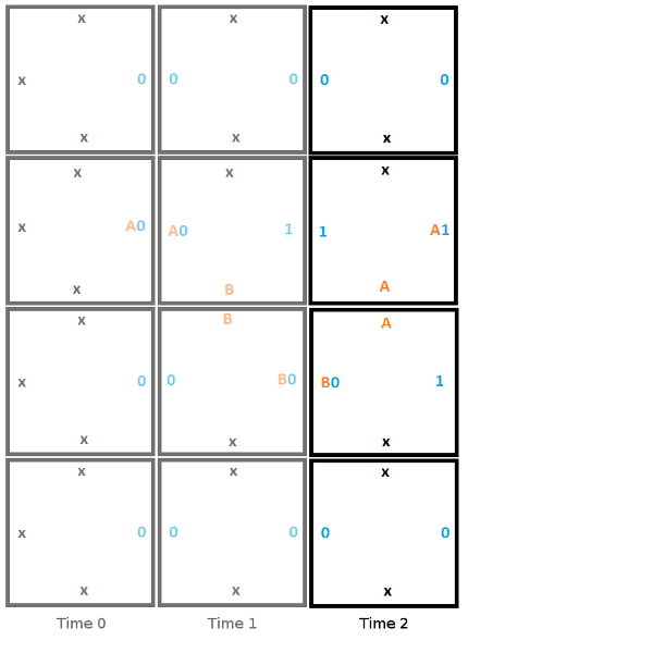
Heres is the second step, where the read reads a 0, writes a 1, moves up, and moves to state A.

Here is the final step, where the head reads a 1 and enters the halt state, signifying that the program has terminated.

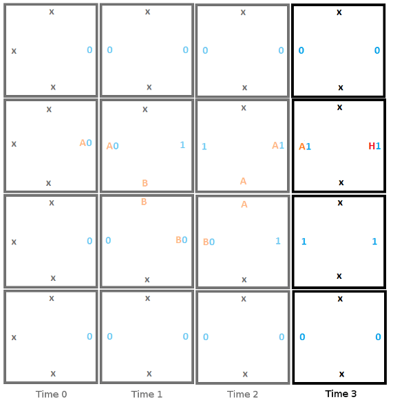
The program halted, and gave an output value of “0110” or 6. This output isn’t really meaningful but other programs can give output that is meaningful. For instance you could have a Turing machine add two numbers, and the output would be the sum of those two numbers.

An Important Detail

There is an important detail that the above doesn’t address, and that many explanations of Wang tile Turing machines don’t seem to talk about.

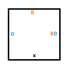
When placing the second tile for time 2, the only constraint from the edges is that the tile must have an x on top and a 1 on the left. This actually makes it ambiguous which tile should be chosen between the two tiles below.

How do we choose the right one then?

The answer is that you make a guess and just choose one. If the wrong one was chosen in this case, when we moved to the next tile, we’d be looking for a tile which had an x on top and a B0 on the left. There is no such tile so you’d be unable to place a tile. When this happened, you’d take a step back to the last tile, and try one of the other possibilities.

So, unfortunately there is some literal trial and error involved when simulating Turing machines with Wang tiles, but it is fairly manageable at least. It definitely makes it a bit more complex to calculate in a pixel shader if you were so inclined (or other massively parallel processing units), but it shouldn’t be that much more costly.

Closing & Links

Some of the links below talk about Wang tiles and Turing machines, but don’t seem to strictly be Turing machines anymore. For instance, you might notice that some examples allow data to travel “back in time” where after the program halts, the answer is in the tape at time 0 of the Turing machine, even though that data wasn’t actually there at time 0. This shows that Wang tiles can do computation in their own right, beyond simulating Turing machines, but I’m not really sure what that technique itself would be called.

Also if you are wondering if this is useful to do computation with Wang tiles, I’m not really sure of any practical usage cases myself. However, apparently scientists have found that DNA can act much like Wang tiles act, where they will fit together only if edges are compatible. Because of this, there is ongoing research into DNA based computation that is based on the work of Wang tile computation. pretty interesting stuff!

Here is a shadertoy implementation of wang tiles computing prime numbers in a webgl pixel shader:
Shadertoy: WangTiles : PrimeGenerator

Here are some great videos on Turing machines and the halting problem:
Turing Machines Explained – Computerphile
Turing & The Halting Problem – Computerphile

Here are some other links:
Computing With Tiles
Wikipedia: Wang Tile
Wang Tiles and Turing Machines
Wang Tiles – 1

Here are some academic papers:
Computing With Tiles
Computability of Tilings

Matrix Form of Bezier Curves

Bezier curves are most often talked about either in terms of the De Casteljau algorithm, or in terms of a mathematical function (Bernstein Polynomials).

Every now and then though, you see people talking about Bezier curves being calculated via matrices. If you ever wondered what that was all about, this post should hopefully explain and demystify that a bit.

If you don’t know how to come up with the equation of a Bezier curve for any number of control points, you should give this a read first:
Easy Binomial Expansion & Bezier Curve Formulas

And if you are curious about the De Casteljau algorithm, you can learn about that here:
The De Casteljau Algorithm for Evaluating Bezier Curves

Ok, all read up on that stuff? Let’s get talking about Bezier curves in matrix form! There are shadertoy links at the end with working wegl glsl demos that include source code.

Making the Matrix Form of Bezier Curves

Coming up with the matrix for a Bezier curve is surprisingly easy. Keep in mind the matrix we are making is for glsl which is a column major matrix order, so you might have to adjust things if you are using a row major matrix order setup (mostly, just transpose the matrix).

The first step is to get the formula for a Bezier curve. We’ll work through the example using a quadratic Bezier curve with 3 control points A,B,C, so we start with the formula below:

f(t) = A*(1-t)^2 + B*2t(1-t) + C*t^2

The next step is to break the equation into one equation per term. Each term has a control point, so we are basically splitting the formula up so that we have one formula per control point.

A*(1-t)^2 \\ B*2t(1-t) \\ C*t^2

Next, we remove the control points and expand each term to get:

1-2t+t^2 \\ 2t-2t^2 \\ t^2

Now, explicitly values of all powers of t that are present:
1*t^0-2*t^1+1*t^2 \\ 0*t^0+2*t^1-2*t^2 \\ 0*t^0+0*t^1+1*t^2

Now the final step. Take the constants that multiply your powers of t and make a matrix out of them. You are done!

\begin{bmatrix} 1 & -2 & 1 \\ 0 & 2 & -2 \\ 0 & 0 & 1 \\ \end{bmatrix}

Using the Matrix Form

Using the matrix form of Bezier curves is also pretty simple.

First, we need to make a vector of the power series of our t value:

powerSeries = \begin{bmatrix} t^0 & t^1 & t^2 \\ \end{bmatrix}

Which can also be written as:

powerSeries = \begin{bmatrix} 1 & t & t^2 \\ \end{bmatrix}

You also need a vector of your control points:

controlPoints = \begin{bmatrix} A & B & C \\ \end{bmatrix}

You next perform this operation to get a result vector:

result = powerSeries * curveMatrix * controlPoints

Then, you add up all components of result to get the value of the curve at time t.

value = result[0] + result[1] + result[2]

All done!

Note that this is a one dimensional Bezier curve. You need to do this operation once per axis to get your final multi dimensional Bezier curve point.

If you are confused by that last line, check out this post: One Dimensional Bezier Curves

Multiplying the Control Points In

You might notice that if you are evaluating several points on the same curve that you are going to be multiplying the curveMatrix matrix by the controlPoints vector over and over. You can multiply the control points into the Bezier curve matrix to make the specific matrix for those control points if you want to. You multiply the columns of the matrix by the control points, and adjust the result calculation like the below.

// Multiply the control points into the curve matrix
curveMatrix[0] *= A;
curveMatrix[1] *= B;
curveMatrix[2] *= C;

// Use the curve matrix that has the control points baked in, to do less math to get the result vector.
// You would calculate the curve matrix once and re-use it multiple times of course!
vec3 result = powerSeries * curveMatrix;
float value = result.x + result.y + result.z;

Closing

You might wonder when you’d use the matrix form. One time to use the matrix form would be when you had fast matrix math support (like on the GPU). Another time to use the matrix form though is if you ever want to cut up a Bezier curve into multiple smaller sub curves. The matrix form can help make that easier, and you can read more about that here if you want: A Matrix Formulation of the Cubic Bezier Curve

Here are some shadertoys that show this all working in webgl/glsl pixel shaders, along with source code:

Shadertoy: 1D Linear Bezier Matrix Form
Shadertoy: 1D Quadratic Bezier Matrix Form
Shadertoy: 1D Cubic Bezier Matrix Form

Actually Making Signed Distance Field Textures With JFA

This post is an addendum to the last post where I say that you can make distance field textures with JFA but don’t fully explain how to make SIGNED distance field textures, which is what you really want.

If you want to go straight to a working demo with webgl pixel shader source code, here is the shadertoy: Shadertoy: JFA SDF Texture

If you naively use a distance transform to make a distance field texture, you’ll get an UNSIGNED distance field texture, where you only have the distance to the surface of the object from the outside, but won’t have the distance to the surface of the object from the inside.

This is important because signed distance field textures have both, and use bilinear interpolation of distance on each side of the shape surface to make a nice smooth line. Below is what happens when you try to use an unsigned distance field texture (aka the distance transform of the image, using JFA / Voronoi information), using the zero distance line as the surface of the object:

It looks ok (if not fairly pixelated), but you can really see it break down when you zoom in:

So you might say to yourself, maybe i need to keep the surface line at distance 0.5 instead of 0.0 so that there is distance information to interpolate? If you do that, the first thing you might notice is that the objects get fatter:

But it does look better when you zoom in, which is a plus:

The real issue is that you really just need the distance from each pixel to the surface of the object from both the inside and the outside. In our case, our Voronoi diagram we make with JFA only gives the distance from the outside. So what is the solution? At first I was thinking maybe you can get the gradient of this data at the point of each pixel and “push the zero line in” a little bit to give at least one pixel layer worth of inside data. However, a brilliant friend of mine came up with the actual solution: You invert your source data so empty space becomes seed, and seed becomes empty space, and you run JFA again to get the distance from the inside!

That actually works very well. It’s also very easy to combine them. You make a pixel shader that reads the data from the outside Voronoi diagram and the inside Voronoi diagram, calculate the output distance (0.5 + outsideDistance * 0.5 – insideDistance * 0.5), and output that 0 to 1 distance value in one or more of the color channels.

Here’s a glsl excerpt below, note that we divide the distance by 8 and clamp between 0 and 1 so that the data is suitable for a normalized color image (normalized as in the color channels can store values between 0 and 1):

// calculate distances from seed coordinates
float outsideDist = clamp(length(outsideSeedCoord-fragCoord) / 8.0, 0.0, 1.0);
float insideDist  = clamp(length(insideSeedCoord-fFragCoord)  / 8.0, 0.0, 1.0);
    
// calculate output distance
float signedDistance = 0.5 + outsideDist * 0.5 - insideDist * 0.5;
        
// set the color based on that distance
fragColor = vec4(signedDistance);

It actually looks a lot like the first image where we use the zero distance line of the unsigned distance field texture, so we still aren’t quite there:

When you zoom in, it looks a little better, but something still seems a bit off:

The final step to making this look good is to realize that the power of signed distance textures is in their ability to interpolate distance information well. When we have a full resolution texture, there is no interpolation going on. We actually need to decrease the size of our distance field texture to make it look better. If only all problems were solved by making textures smaller!

Here is the resulting image when making the distance field texture 1/4 as large on each axis (1/16th as big total):

And zooming in you can see that it scales very well. The zoom is a 20x magnification, on top of the magnification we already get from it being a larger texture:

And just to show the intermediary textures, here is the outside distance Voronoi diagram:

And the inside distance Voronoi diagram (The seed is in bright green, the dim green is the empty space that has distance information):

And here is the final distance field texture used to render the final result I showed above.

Zoomed in to show just how low resolution it is! This is the thing that looks like a + or a sword just left of middle.

Again, here is the shadertoy that does this technique, generating a signed distance field texture on the fly for randomly placed objects, and then using that signed distance field to render a larger image that you can further zoom in to:
Shadertoy: JFA SDF Texture

Fast Voronoi Diagrams and Distance Field Textures on the GPU With the Jump Flooding Algorithm

The image below is called a Voronoi diagram. The circles show you the location of the seeds and the color of each pixel represents the closest seed to that pixel. The value of this diagram is that at any point on the image, you can know which seed (point) is the closest to that pixel. It’s basically a pre-computed “closest object” map, which you can imagine some uses for I bet.

Voronoi diagrams aren’t limited to just points as seeds though, you can use any shape you want.

One way Voronoi diagrams can be useful is for path finding because they are dual to (the equivelant of) Delauny triangulation (More info at How to Use Voronoi Diagrams to Control AI).

Another way they can be useful is in generating procedural content, like in these shadertoys:
Shadertoy: Voronoi – rocks
Shadertoy: Voronoi noises

Another really cool usage case of Voronoi diagrams is in creating what is called the “Distance Transform”. The distance transform calculates and stores the distance from each pixel to the closest seed, whichever one that may be. Doing that, you may get an image like this (note that the distance is clamped at a maximum and mapped to the 0 to 1 range to make this image).

That is what is called a distance texture and can be used for a very cool technique where you have texture based images that can be zoomed into / enlarged quite a ways before breaking down and looking bad. The mustache in the image below was made with a 32×16 single channel 8bpp image for instance! (ignore the white fog, this was a screenshot from inside a project I was working on)

Distance field textures are the next best thing to vector graphics (great for scalable fonts in games, as well as decals!) and you can read about it here: blog.demofox.org: Distance Field Textures

Now that you know what Voronoi diagrams and distance transforms are used for, let’s talk about one way to generate them.

Jump Flooding Algorithm (JFA)

When you want to generate either a Voronoi diagram or a distance transform, there are algorithms which can get you the exact answer, and then there are algorithms which can get you an approximate answer and generally run a lot faster than the exact version.

The jump flooding algorithm is an algorithm to get you an approximate answer, but seems to have very little error in practice. It also runs very quickly on the GPU. It runs in constant time based on the number of seeds, because it’s execution time is based on the size of the output texture – and is based on that logarithmically.

Just a real quick note before going into JFA. If all else fails, you could use brute force to calculate both Voronoi diagrams as well as distance transforms. You would just loop through each pixel, and then for each pixel, you would loop through each seed, calculate the distance from the pixel to the seed, and just store the information for whatever seed was closest. Yes, you even do this for seed pixels. The result will be a distance of 0 to the seed 😛

Back to JFA, JFA is pretty simple to program, but understanding why it works may take a little bit of thinking.

Firstly you need to prepare the N x N texture that you want to run JFA on. It doesn’t need to be a square image but let’s make it square for the explanation. Initialize the texture with some sentinel value that means “No Data” such as (0.0, 0.0, 0.0, 0.0). You then put your seed data in. Each pixel that is a seed pixel needs to encode it’s coordinate inside of the pixel. For instance you may store the fragment coordinate bitpacked into the color channels if you have 32 bit pixels (x coordinate in r,g and y coordinate in b,a). Your texture is now initialized and ready for JFA!

JFA consists of taking log2(N) steps where each step is a full screen pixel shader pass.

In the pixel shader, you read samples from the texture in a 3×3 pattern where the middle pixel is the current fragment. The offset between each sample on each axis is 2^(log2(N) – passIndex – 1), where passIndex starts at zero.

That might be a bit hard to read so let’s work through an example.

Let’s say that you have an 8×8 texture (again, it doesn’t need to be square, or even power of 2 dimensions, but it makes it easier to explain), that has a 16 bit float per RGBA color channel. You fill the texture with (0.0, 0.0, 0.0, 0.0) meaning there is no data. Let’s say that you then fill in a few seed pixels, where the R,G channels contain the fragment coordinate of that pixel. Now it’s time to do JFA steps.

The first JFA step will be that for each pixel you read that pixel, as well as the rest of a 3×3 grid with offset 4. In total you’d read the offsets:
(-4.0, -4.0), (0.0, -4.0), (4.0, -4.0),
(-4.0, 0.0), (0.0, 0.0), (4.0, 0.0),
(-4.0, 4.0), (0.0, 4.0), (4.0, 4.0)

For each texture read you did, you calculate the distance from the seed it lists inside it (if the seed exists aka, the coordinate is not 0,0), and store the location of the closest seed int the output pixel (like, store the x,y of the seed in the r,g components of the pixel).

You then do another JFA step with offset 2, and then another JFA step with offset 1.

JFA is now done and your image will store the Voronoi diagram, that’s all! If you look at the raw texture it won’t look like anything though, so to view the Voronoi diagram, you need to make a pixel shader where it reads in the pixel value, deocdes it to get the x,y of the closest seed, and then uses that x,y somehow to generate a color (use it as a seed for a prng for instance). That color is what you would output in the pixel shader, to view the colorful Voronoi diagram.

To convert the Voronoi diagram to a distance transform, you’d do another full screen shader pass where for each pixel you’d calculate the distance from that pixel to the seed that it stores (the closest seed location) and write the distance as output. If you have a normalized texture format, you’re going to have to divide it by some constant and clamp it between 0 and 1, instead of storing the raw distance value. You now have a distance texture!

More Resources

I originally came across this algorithm on shadertoy: Shadertoy: Jump Flooding. That shadertoy was made by @paniq who is working on some pretty interesting stuff, that you can check out both on shadertoy and twitter.

The technique itself comes from this paper, which is a good read: Jump Flooding in GPU with Applications to Voronoi Diagram and Distance Transform

Extensions

While JFA as explained is a 2D algorithm, it could be used on volume textures, or higher dimensions as well. Higher dimensions mean more texture reads, but it will still work. You could render volume textures with raymarching, using the distance information as a hint for how far you could march the ray each step.

Also, I’ve played around with doing 5 reads instead of 9, doing a plus sign read instead of a 3×3 grid. In my tests it worked just as well as regular JFA, but I’m sure in more complex situations there are probably at least minor differences. Check the links section for a shadertoy implementation of this. I also tried doing a complete x axis JFA followed by a y axis JFA. That turned out to have a LOT of errors.

You can also weight the seeds of the Voronoi diagram. When you are calculating the distance from a pixel to a seed point, you use the seed weight to multiply and/or add to the distance calculated. You can imagine that perhaps not all seeds are created equal (maybe some AI should avoid something more than something else), so weighting can be used to achieve this.

Shadertoys

Here are some shadertoys I made to experiment with different aspects of this stuff. You can go check them out to see working examples of JFA in action with accompanying glsl source code.

Jump Flood Algorithm: Points – Point Seeds
Jump Flood Algorithm: Shapes – Shape Seeds
Jump Flood Algorithm: Weight Pts – Multiplicative Weighting
Jump Flood Algorithm: Add Wt Pts – Additive Weighting
Separable Axis JFA Testing – Does 5 reads instead of 9, also shows how separating axis completely fails.

Here is a really interesting shadertoy that shows a way of modifying a Vornoi diagram on the fly: Shadertoy: zoomable, stored voronoi cells

GPU Texture Sampler Bezier Curve Evaluation

Below is a paper I submitted to jcgt.org that unfortunately did not get accepted. Maybe next time!

The main idea of this paper is that bilinear interpolation can be equivalent to the De Casteljau algorithm, which means that if you set up a texture in a specific way, and sample from it at specific texture coordinates, that it will in fact give you Bezier curve points as output! It scales up for higher dimensional textures, as well as higher order curves.

The image below shows this in action for a cubic Bezier curve (3 control points) being stored and recalled from a 2×2 texture (there is actually a curve stored in each color channel).

This image is from an extension linked to lower down which applies the technique to surfaces and volumes:

The primary feedback from the reviewers and editor was that:

  • It was an interesting technique and they thought it was a paper worth reading.
  • The usage case was fairly limited though – basically only when your are compute bound in your shader program, and have some curve calculations to offload to the texture sampler. Or if you are already using a lookup texture and would benefit from fewer instructions and smaller lookup textures.
  • It could have been shorter due to the writing being shorter, but also it could have been less thorough. For instance, it didn’t need to show equivalence to both the De Casteljau’s algorithm as well as Bernstein polynomials, since it’s already known that those are equivalent.
  • They wanted some more performance details

I agree with the feedback, and don’t feel like taking the time to change and resubmit or submit else where, so I’m sharing it here on my blog. I hope you enjoy it and find it interesting (:

Here is the paper:
GPUBezier2016.pdf

Here is the supplemental materials (opengl and webgl source code):
SupplementalMaterials.zip

Here is the webgl demo from the supplemental materials, hosted on my site:
GPU Efficient Texture Based Bezier Curve Evaluation

Here are some working shadertoy demos of the technique:
Shadertoy: Mystery Curves – Quadratic
Shadertoy: Mystery Curves – Cubic
Shadertoy: Mystery Curves – Quartic
Shadertoy: Mystery Curves – Quintic

Extensions

Continuations of this work:

Failed Experiments

Continuations that didn’t work out:

What are your thoughts? Is this cool? Is it lame? Got some ideas to improve it? Leave a comment! (:

G-Buffer Upsizing

The other day I had a thought:

Rendering smaller than full screen images is super helpful for performance, but upsizing an image results in pretty bad quality vs a full resolution render.

What if instead of upsizing the final rendered image, we upsized the values that were used to shade each pixel?

In other words, what if we rendered a scene from a less than full resolution g-buffer?

I was thinking that could be useful in doing ray based graphics, not having to trace or march quite so many rays, but also perhaps it could be useful for things like reflections where a user isn’t likely to notice a drop in resolution.

I’m sure I’m not the first to think of this, but I figured I’d explore it anyways and see what I could see.

I made an interactive shadertoy demo to explore this if you want to see it first hand:
Shadertoy: G-Buffer Upsizing

Result

In short, it does look better in a lot of ways because the normals, uv coordinates and similar parameters interpolate really well, but the edges of shapes are aliased really bad (jaggies).

Check out the images below to see what i mean. The first image is a full sized render. The second image is a 1/4 sized render (half x and half y resolution). The third image is a 1/16th sized render (quarter x and quarter y resolution)


For comparison, here’s a 1/4 sized and 1/16 sized render upsized using bicubic IMAGE interpolation instead of g-buffer data interpolation:


Details & More Information

Despite the aliased results at 1/16th render size, this seems like it may be a reasonable technique at larger render sizes, depending on the level of quality you need. Doing half vertical or half horizontal resolution looks very close to the full sized image for instance. The edges are a tiny bit more aliased along one direction, but otherwise things seem decent:

Since the g-buffer has only limited space, you will probably want to bit pack multiple fields together in the same color channels. When you do that, you throw out the possibility of doing hardware interpolation unfortunately, because it interpolates the resulting bit packed value, not the individual fields that you packed in.

Even when doing the interpolation yourself in the pixel shader, for the most part you can really only store information that interpolates well. For instance, you could store a diffuse R,G,B color, but you wouldn’t want to store and then interpolate a material index. This is because you might have material index 10 (say it’s blue) next to material index 0 (say it’s green), and then when you interpolate you could end up with material index 5 which may be red. You’d get red between your blue and green which is very obviously wrong.

In my demo I did have a material index per pixel, but i just used nearest neighbor for that particular value always. To help the appearance of aliasing, I also stored an RGB diffuse color that i interpolated.

I stored the uvs in the g-buffer and sampled the textures themselves in the final shader though, to make sure and get the best texture information I could. This makes textures look great at virtually any resolution and is a lot of the reason why the result looks as good as it does IMO.

The fact that normals interpolate is a good thing, except when it comes to hard edges like the edge of the cube, or at the edge of any object really. In the case of the cube edge, it smooths the edge a little bit, making a surface that catches specular lighting and so highlights itself as being incorrect (!!). In the case of the edge of regular objects, a similar thing happens because it will interpolate between the normal at the edge of the object and the background, making a halo around the object which again catches specular lighting and highlights itself as being incorrect.

I think it could be interesting or fruitful to explore using edge detection to decide when to blend or not, to help the problem with normals, or maybe even just some edge detection based anti aliasing could be nice to make the resulting images better. The depth (z buffer value) could also maybe be used to help decide when to interpolate or not, to help the problem of halos around every object.

Interestingly, bicubic interpolation actually seems to enhance the problem areas compared to bilinear. It actually seems to highlight areas of change, where you would actually want it to sort of not point out the problems hehe. I think this is due to Runge’s phenomenon. Check out the depth information below to see what i mean. The first is bilinear, the second is bicubic:


One final side benefit of this I wanted to mention, is that if you are doing ray based rendering, where finding the geometry information per pixel can be time consuming, you could actually create your g-buffer once and re-shade it with different animated texture or lighting parameters, to give you a constant time (and very quick) render of any scene of any complexity, so long as the camera wasn’t moving, and there were no geometry changes happening. This is kind of along the same lines as the very first post I made to this blog about 4 years ago, which caches geometry in screen space tiles, allowing dirty rectangles to be used (MoriRT: Pixel and Geometry Caching to Aid Real Time Raytracing).

Anyone else go down this path and have some advice, or have any ideas on other things not mentioned? (:

Next up I think I want to look at temporal interpolation of g-buffers, to see what sort of characteristics that might have. (Quick update, the naive implementation of that is basically useless as far as i can tell: G-Buffer Temporal Interpolation).

Related Stuff

On shadertoy, casty mentioned that if you have some full res information, and some less than full res information, you can actually do something called “Joint Bilateral Upsampling” to get a better result.

Give this paper a read to learn more!
Joint Bilateral Upsampling

It turns out someone has already solved this challenge with great success. They use “the MSAA trick” to get more samples at the edges. Check out ~page 38:
GPU-Driven Rendering Pipelines

Simplifying Boolean Expressions With Karnaugh Maps

Karnaugh maps are a formalized way of turning a truth table into a fairly minimal logical expression.

It’s fairly minimal in that it’s the minimal “sum of products” representation, but that might not be the minimal representation of the logic circuit.

The sum of products representation just means that you OR (sum) multiple terms that are ANDed (product) together. For instance the below is a sum of products expression:

Out = \overline{A}B + AB

With multiplication being AND, addition being OR, and a line over a letter being a NOT, the above could be written in C++ code like this:

bool out = (!A && B) || (A && B);

It would be real easy to write code like that especially if you were adding onto an existing condition, and you might not even notice that it isn’t the minimal Boolean expression to make the desired output.

Using Boolean algebra, you can do the following simplifications:
Out = \overline{A}B + AB\\ = B*(\overline{A}+A)\\ = B*1\\ = B

Which simplifies the C++ code to just this:

bool out = B;

Using Boolean algebra to simplify, you’d have to remember (or derive) the identity that A+\overline{A}=1 , and all the other identities to help you simplify equations.

Karnaugh maps make this easier because you will be able to see visually what can be combined (simplified) and what can’t.

Again though, while they give you the smallest possible sum of products representation of the logic circuit, that may not be the smallest possible representation of the circuit.

Let’s get to it!

Two Variable Karnaugh Map: Basics

Going with the example above, it takes two Boolean variables as input (A and B), and gives one Boolean variable as output. Having two input variables means we need a two variable Karnaugh map.

The first step to building the Karnaugh map is having a truth table for the input to output mappings. For our example we’ll use this truth table. This is one of many truth tables that satisfies our equation, so we are working backwards a bit, but hopefully it still makes sense. Usually you would start with the truth table and get a Boolean equation, not the other way around.
\begin{array}{c|c|c} A & B & Out\\ \hline 0 & 0 & 0 \\ 0 & 1 & 1 \\ 1 & 0 & 0 \\ 1 & 1 & 1 \\ \end{array}

The next thing we do is make our karnaugh map by making a square 2×2 grid where one side of the square is the possible A values, the other side is the possible B values, and the contents of the grid cells are the values we want the formula to come out to be:

\begin{array}{ccc} & \overline{B} & B \\ \overline{A} & 0 & 1 \\ A & 0 & 1 \\ \end{array}

Next, what you do is circle all 1’s that are in groups of a power of two (one item or two items). Doing that, we get this:

\begin{array}{ccc} & \overline{B} & B \\ \cline{3-3} \overline{A} & 0 & \multicolumn{1}{|c|}{1} \\ A & 0 & \multicolumn{1}{|c|}{1} \\ \cline{3-3} \end{array}

Looking at what we circled, we can see that both values of A are involved in our group, so A doesn’t matter to the output. We can also see that \overline{B} is not involved in any places where there is a 1, so we can ignore that too. All that leaves is B, which is our final, and most minimal answer.

That agrees with the Boolean algebra solution, but came without having to remember any identities. Hooray!

Two Variable Karnaugh Map: Overlaps

If there were multiple groups, you would combine each group with OR to get the final answer. Groups are also allowed to overlap! For instance, let’s look at this truth table to start out:

\begin{array}{c|c|c} A & B & Out\\ \hline 0 & 0 & 0 \\ 0 & 1 & 1 \\ 1 & 0 & 1 \\ 1 & 1 & 1 \\ \end{array}

Turning that into a Karnaugh map, we get this:

\begin{array}{ccc} & \overline{B} & B \\ \overline{A} & 0 & 1 \\ A & 1 & 1 \\ \end{array}

Next when it’s time to circle our groups, we have two groups, and they overlap! Here is the first group, which is the same as before:

\begin{array}{ccc} & \overline{B} & B \\ \cline{3-3} \overline{A} & 0 & \multicolumn{1}{|c|}{1} \\ A & 1 & \multicolumn{1}{|c|}{1} \\ \cline{3-3} \end{array}

That group can be expressed as just B.

The other group is this:

\begin{array}{ccc} & \overline{B} & B \\ \overline{A} & 0 & 1 \\ \cline{2-3} A & \multicolumn{1}{|c}{1} & \multicolumn{1}{c|}{1} \\ \cline{2-3} \end{array}

That group can be expressed as just A.

Lastly, we OR our groups together, aka we sum our products, and we get A+B 
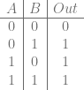
as an answer, which in other words is just A OR B. Check out the truth table and you can see that it is indeed a truth table for OR!

Two Variable Karnaugh Map: Single Sized Groups

What if we don’t have groups of two though, what if we only have groups of one? Let’s explore that real quick with the following truth table:

\begin{array}{c|c|c} A & B & Out\\ \hline 0 & 0 & 1 \\ 0 & 1 & 0 \\ 1 & 0 & 0 \\ 1 & 1 & 1 \\ \end{array}

That becomes this Karnaugh map:

\begin{array}{ccc} & \overline{B} & B \\ \overline{A} & 1 & 0 \\ A & 0 & 1 \\ \end{array}

We once again have two groups, but they are each of size one, which is totally ok!

The upper left group is expressed as \overline{AB}
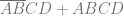
, while the lower right group is expressed as AB. We OR those two groups together to get the answer: \overline{AB} + AB. That’s all there is to it.

Four Variable Karnaugh Map: Don’t Care Values

Let’s get a little more sophisticated and see how we would handle four input variables (We could go to three variables next but after learning two and four it’ll be easy to see how to do three). We will start with a truth table, but our truth table will only contain the input values we care about. We’ll omit the ones we don’t care about.

\begin{array}{c|c} ABCD & Out\\ \hline 0001 & 0 \\ 0011 & 1 \\ 0111 & 0 \\ 1111 & 1 \\ \end{array}

We’ll put 1’s and 0’s into the Karnaugh map to match our truth table, but put x’s where the output wasn’t listed. These are “don’t care” values, where they could either be 0’s or 1’s, depending on whichever is more convinient for us when simplifying. We are also going to change how we label the map a bit.

\begin{array}{cccccc} & & \multicolumn{4}{c}{CD} \\ & & 00 & 01 & 11 & 10 \\ & 00 & x & 0 & 1 & x \\ AB & 01 & x & x & 0 & x \\ & 11 & x & x & 1 & x \\ & 10 & x & x & x & x \\ \end{array}

In this case, even with the wild card don’t care values, we still just have two 1 item groups, that we OR together to get the answer:

\overline{AB}CD+ABCD

Note that we could factor out the CD and make it into the below, but then it would no longer be in a sum of products form.

CD(\overline{AB}+AB)

You might also have noticed the strange ordering of the values in the table: 00, 01, 11, 10. Normally doesn’t 2 (10) come before 3 (11)? It does, except in this case, we only want to change one variable at a time between neighboring cells. Going from 01 to 11 means that the first bit changed, while going from 01 to 10 means that two bits changed, so isn’t useful for us finding groups. The order that the numbers are in is actually called Gray Code, named after Frank Grey (Wikipedia: Gray Code).

Four Variable Karnaugh Map: Larger Groups

When dealing with karnaugh maps, like I said before, the groups have to be a size of a power of two, but interestingly it can be a power of two on each axis. So valid groups include 4×1, 2×1, 2×2, 4×2 and others. Let’s take a look at one where we encounter a 2×2 group.

Let’s start with the truth table:

\begin{array}{c|c} ABCD & Out\\ \hline 0000 & 0 \\ 0001 & 0 \\ 0010 & 0 \\ 0011 & 0 \\ 0100 & 0 \\ 0101 & 1 \\ 0110 & 0 \\ 0111 & 1 \\ 1000 & 0 \\ 1001 & 0 \\ 1010 & 0 \\ 1011 & 1 \\ 1100 & 0 \\ 1101 & 1 \\ 1110 & 0 \\ 1111 & 1 \\ \end{array}

That gives us the Karnaugh map:

\begin{array}{cccccc} & & \multicolumn{4}{c}{CD} \\ & & 00 & 01 & 11 & 10 \\ & 00 & 0 & 0 & 0 & 0 \\ AB & 01 & 0 & 1 & 1 & 0 \\ & 11 & 0 & 1 & 1 & 0 \\ & 10 & 0 & 0 & 1 & 0 \\ \end{array}

There are two groups there. The first is the 2×2 group below and is the intersection of where B is 1, and D is 1, so can be represented as BD.

\begin{array}{cccccc} & & \multicolumn{4}{c}{CD} \\ & & 00 & 01 & 11 & 10 \\ & 00 & 0 & 0 & 0 & 0 \\ \cline{4-5} AB & 01 & 0 & \multicolumn{1}{|c}{1} & \multicolumn{1}{c|}{1} & 0 \\ & 11 & 0 & \multicolumn{1}{|c}{1} & \multicolumn{1}{c|}{1} & 0 \\ \cline{4-5} & 10 & 0 & 0 & 1 & 0 \\ \end{array}

The second group is a 1×2 group that overlaps the first, and is where A,C and D are 1, but B can be either 0 or 1. That makes it able to be represented as ACD.

\begin{array}{cccccc} & & \multicolumn{4}{c}{CD} \\ & & 00 & 01 & 11 & 10 \\ & 00 & 0 & 0 & 0 & 0 \\ AB & 01 & 0 & 1 & 1 & 0 \\ \cline{5-5} & 11 & 0 & 1 & \multicolumn{1}{|c|}{1} & 0 \\ & 10 & 0 & 0 & \multicolumn{1}{|c|}{1} & 0 \\ \cline{5-5} \end{array}

We combine those groups with OR to get the answer:

BD+ACD

Four Variable Karnaugh Map: Wrap Around

Interestingly, you can make groups by wrapping around the edges of the Karnaugh map, either horizontally or vertically. Let’s start with a truth table:

\begin{array}{c|c} ABCD & Out\\ \hline 0000 & 0 \\ 0001 & 0 \\ 0010 & 0 \\ 0011 & 1 \\ 0100 & 0 \\ 0101 & 0 \\ 0110 & 0 \\ 0111 & 0 \\ 1000 & 0 \\ 1001 & 0 \\ 1010 & 0 \\ 1011 & 1 \\ 1100 & 0 \\ 1101 & 0 \\ 1110 & 0 \\ 1111 & 0 \\ \end{array}

That gives us the Karnaugh map:

\begin{array}{cccccc} & & \multicolumn{4}{c}{CD} \\ & & 00 & 01 & 11 & 10 \\ & 00 & 0 & 0 & 1 & 0 \\ AB & 01 & 0 & 0 & 0 & 0 \\ & 11 & 0 & 0 & 0 & 0 \\ & 10 & 0 & 0 & 1 & 0 \\ \end{array}

Here is the group highlighted below, which is represented as \overline{B}CD, which is also the answer:

\begin{array}{cccccc} & & \multicolumn{4}{c}{CD} \\ & & 00 & 01 & 11 & 10 \\ & 00 & 0 & 0 & \multicolumn{1}{|c|}{1} & 0 \\ \cline{5-5} AB & 01 & 0 & 0 & 0 & 0 \\ & 11 & 0 & 0 & 0 & 0 \\ \cline{5-5} & 10 & 0 & 0 & \multicolumn{1}{|c|}{1} & 0 \\ \end{array}

Two Variable Karnaugh Map: Handling Redundant Info

If you are like me, you might be wondering – If Karnaugh maps can give you the minimal sum of products expression for a truth table, how does it deal with redundant information or solutions that are of equal size, so it’s ambiguous which to choose?

For instance, Let’s go with the truth table table below. All other inputs not listed are “don’t care” values.

\begin{array}{c|c} AB & Out\\ \hline 00 & 0 \\ 11 & 1 \\ \end{array}

It’s obvious that the output bit corresponds exactly to both A and B separately. Which one does it choose, or does it make some more complex expression that involves both?

Here is the Karnaugh map:

\begin{array}{ccc} & \overline{B} & B \\ \overline{A} & 0 & x \\ A & x & 1 \\ \end{array}

Well, the disambiguation comes up now that you – the pattern finder in the Karnaugh map – chooses between the two possible groups.

One answer, which is perfectly valid is the below, which is just A.

\begin{array}{ccc} & \overline{B} & B \\ \overline{A} & 0 & x \\ \cline{2-3} A & \multicolumn{1}{|c}{x} & \multicolumn{1}{c|}{1} \\ \cline{2-3} \end{array}

The other answer, which is also perfectly valid, is the below, which is just B

\begin{array}{ccc} & \overline{B} & B \\ \cline{3-3} \overline{A} & 0 & \multicolumn{1}{|c|}{x} \\ A & x & \multicolumn{1}{|c|}{1} \\ \cline{3-3} \end{array}

So, the disambiguation / simplification is left up to the user to choose, but yes, it still comes up with a minimal sum of products answer, and doesn’t try to incorporate both bits into a more complex logic operation.

Other Notes

The act of turning a truth table into a logical expression is called logical synthesis, if you want to read more along those lines.

You might be wondering if because there is a sum of products form, if there is also a product of sums form? There is in fact, and you can get that form from Karnaugh maps as well. It may result in a more optimal logical expression. More info on that here: Is Karnaugh Map possible for Maxterms?.

You might be tempted to bring a higher number of variables into the mix. Be warned… adding a 5th variable makes the Karnaugh map into a 4x4x2 3d shape. Adding a 6th variable makes it into a 4x4x4 cube. Adding a 7th variable makes it into a 4x4x4x2 hypercube, and the pattern continues.

For higher numbers of inputs, people will often use a different algorithm instead, that I hope to write a post on before too long. You can read about it here: Wikipedia: Quine–McCluskey algorithm

Lastly, you might be wondering, what do i do if i have M input bits, and N output bits? How can I make a circuit or a set of instructions to generate a minimal logical expression to encompass that?

Well, one simple way is to handle each bit separately and have N Karnaugh maps each having M variables. A problem there though is that computers do operations on multiple bits at the same time with most operations, so having each bit do it’s calculations without considering sharing instructions with another bit leaves some efficiency on the table.

I’m not sure of any better algorithms currently, but I’ve asked on stack exchange so there may be some more info there by the time you read this:
Algorithms for logical synthesis of multiple output bits?

What Happens When you Mix Hash Tables and Binary Searching?

While not the most cache friendly operation, binary searching a sorted data set is a pretty good way to search a data set for a specific value because for N items, you have an average case and worst case of O(log N) (Wikipedia: Binary Search Algorithm).

Hashing is also a decent way to do data searching, because it has a best case for search of O(1) with the average case being able to be near that when tuned well, but in practice due to collisions it can get get up to O(n) (Wikipedia: Hash Table).

Note that if you know the keys in advance, you can ALWAYS get O(1) lookup by using the information from the last post: Minimal Perfect Hashing.

One way to deal with hash collisions is to store all the collisions for a specific hash value in a list or array.

For instance, if you had a 4 bit hash, you could have 16 arrays, where the [0]th array stored all the items that hashed to 0, the [1]th array stored all items that hashed to 1 and so on, going up to the [15]th array which stored all items that hashed to 15.

What would happen if we stored the arrays in sorted order and then did a binary search within the buckets? What would that mean to search times?

Interestingly, assuming a good hash function, the answer is that every bit of hash you use subtracts one from the number of tests you’d have to do with binary searching (See footnote 1).

Examples

For instance, let’s say you had 1024 items sorted in an array, you would have to do up to 10 tests to search for a value in that array using a binary search since log2(1024)=10 (See footnote 2).

If we use a 1 bit hash, assuming a good hash function, that would split the array into two arrays each having 512 items in it. Those each can take up to 9 tests to search using a binary search since log2(512)=9. Doing the hash to choose which of the two lists to search cuts our search from up to 10 tests, down to 9 tests.

If instead we used a 2 bit hash, we would divide the 1024 item list into four lists each having 256 items in them. Each of these lists can be searched with up to 8 tests since log2(256) = 8. So using a 2 bit hash, we can cut our search down to 8 tests max.

Let’s say that we used an 8 bit hash. That would cut our list up into 256 lists, each of which only has 4 items in it. Each list can be searched with up to 2 tests since log2(4) = 2. Using an 8 bit hash cuts our max number of searches from 10 down to 2!

Let’s say we used a 16 bit hash, what would happen then?

Well, that would mean we had 65536 hash buckets, but only 1024 items to store in the buckets. If we had a best case collision free hash, that means only 1024 buckets had an item in them, and the rest were empty.

You’d have to hash the value you were searching for to get the hash bucket index, and if there was an item there, you’d have to test that item. If there was no item there, you could return that the value wasn’t found.

The hash isn’t free though, so this is basically O(1) or doing 1 test.

So, while each bit of hash subtracts one test from the binary search, it of course can’t go negative, or become free, so it basically has a minimum of 1.

Footnotes

  1. Technically it only approximately subtracts one from the number of tests you’d have to do, even if the hash function divides the list as evenly as possible, due to footnote 2 and not being able to split an odd number of items exactly in half.
  2. technically 1024 items in an array could take up to 11 tests! You can see why with 4 items with indices 0,1,2,3. First you’d test index 2. If the value we were looking for was greater, we’d test 3 and then be done with either a found or not found result. That’s just 2 searches total. But, if the value we were looking for was less than index 2, we’d have to test index 1, and then optionally test index 0 depending on how the search value compared to index 1. With only 3 items, indicies 0,1,2, we test index 1, then either index 0 or 2 and be done, and so only have to test twice. A binary search takes log2(N+1) tests, where N is the number of items you are looking through.

Quick Blurb

The last post i wrote on minimal perfect hashing was insanely popular (by my standards) on both reddit and hacker news. The previous highest number of visitors I had ever had to my blog in one day was about 230, but on the 16th I got 4187 visitors, and on the 17th I got 7277 visitors. That means there were over 10,000 visitors over those two days.

That is nuts!!

As a data point for those who might find it interesting, the bulk of the traffic from the first day was reddit, and the bulk of the traffic from the second day was hacker news.

I also found it interesting to see what all those people looked at after the minimal perfect hashing algorithm.

I’ve learned as the years have gone on so some of my older stuff probably contains more errors than my newer stuff (which is also not error free I’m sure).

Anyways, thanks for reading, and I hope you guys find my writings interesting and useful. Please feel free to comment and correct any misinformation, or let us know about better alternatives (:

O(1) Data Lookups With Minimal Perfect Hashing

Hash tables are great in that you can hash a key and then use that hash as an index into an array to get the information associated with that key. That is very fast, so long as you use a fast hash function.

The story doesn’t end there though because hash functions can have collisions – multiple things can hash to the same value even though they are different. This means that in practice you have to do things like store a list of objects per hash value, and when doing a lookup, you need to do a slower full comparison against each item in the bucket to look for a match, instead of being able to only rely on the hash value comparisons.

What if our hash function didn’t have collisions though? What if we could take in N items, hash them, and get 0 to N-1 as output, with no collisions? This post will talk about how to make that very thing happen, with simple sample C++ code as well, believe it or not!

Minimal Perfect Hashing

Perfect hashing is a hash function which has no collisions. You can hash N items, and you get out N different hash values with no collisions. The number of items being hashed has to be smaller than or equal to the possible values your hash can give as output though. For instance if you have a 4 bit hash which gives 16 possible different hash values, and you hash 17 different items, you are going to have at least one collision, it’s unavoidable. But, if you hash 16 items or fewer, it’s possible in that situation that you could have a hash which had no collisions for the items you hashed.

Minimal perfect hashing takes this a step further. Not only are there no collisions, but when you hash N items, you get 0 to N-1 as output.

You might imagine that this is possible – because you could craft limitless numbers of hashing algorithms, and could pass any different salt value to it to change the output values it gives for inputs – but finding the specific hashing algorithm, and the specific salt value(s) to use sounds like a super hard brute force operation.

The method we are going to talk about today is indeed brute force, but it cleverly breaks the problem apart into smaller, easier to solve problems, which is pretty awesome. It’s actually a pretty simple algorithm too.

Here is how you create a minimal perfect hash table:

  1. Hash the items into buckets – there will be collisions at this point.
  2. Sort the buckets from most items to fewest items.
  3. Find a salt value for each bucket such that when all items in that bucket are hashed, they claim only unclaimed slots. Store this array of salt values for later. it will be needed when doing a data lookup.
  4. If a bucket only has one item, instead of searching for a salt value, you can just find an unclaimed index and store -(index+1) into the salt array.

Once you have your minimal perfect hash calculated, here is how you do a lookup:

  1. Hash the key, and use that hash to find what salt to use.
  2. If the salt is positive (or zero), hash the key again using the salt. The result of that hash will be an index into the data table.
  3. If the salt is negative, take the absolute value and subtract one to get the index in the data table.
  4. Since it’s possible the key being looked for isn’t in the table, compare the key with the key stored at that index in the table. If they match, return the data at that index. If they don’t match, the key was not in the table.

Pretty simple isn’t it?

Algorithm Characteristics

This perfect minimal hash algorithm is set up to be slow to generate, but fast to query. This makes it great for situations where the keys are static and unchanging, but you want fast lookup times – like for instance loading a data file for use in a game.

Interestingly though, while you can’t add new keys, you could make it so you could delete keys. You would just remove the key / value pair from the data set, and then when doing a lookup you’d find an empty slot.

Also, there is nothing about this algorithm that says you can’t modify the data associated with the keys, at runtime. Modifying the data associated with a key doesn’t affect where the key/value pair is stored in the table, so you can modify the data all you want.

If you wanted to be able to visit the items in a sorted order, when searching for the perfect minimal hash, you could also make the constraint that when looking for the salt values, that not only did the items in the bucket map to an unclaimed slot, you could make sure they mapped to the correct slot that they should be in to be in sorted order. That would increase the time it took to generate the table, and increase the chances that there was no valid solution for any salt values used, but it is possible if you desire being able to know the items in some sorted order.

Interestingly, the generation time of the minimal perfect hash apparently grows linearly with the number of items it acts on. That makes it scale well. On my own computer for instance, I am able to generate the table for 100,000 items in about 4.5 seconds.

Also, in my implementation, if you have N items, it has the next lower power of two number of salt values. You could decrease the number of salt values used if you wanted to use less memory, but that would again come at the cost of increased time to generate the table, as well as increase the chances that there was no valid solution for any salt values used.

Example Code

Below is a simple implementation of the algorithm described.

The main point of the code (besides functionality) is readability so it isn’t optimized as well as it could be, but still runs very fast (100,000 items processed in about 4.5 seconds on my machine). Debug is quite a bit slower than release for me though – I gave up on those same 100,000 items after a few minutes running in debug.

The code below uses MurmurHash2, but you could drop in whatever hashing algorithm you wanted.

The data file for this code is words.txt and comes to us courtesy of English Wordlists.

#include <vector>
#include <algorithm>
#include <assert.h>
#include <fstream>
#include <string>

unsigned int MurmurHash2(const void * key, int len, unsigned int seed);

//=================================================================================
template <typename VALUE>
class CPerfectHashTable {
public:

    typedef std::pair<std::string, VALUE> TKeyValuePair;
    typedef std::vector<TKeyValuePair> TKeyValueVector;
    struct SKeyValueVectorBucket {
        TKeyValueVector m_vector;
        size_t          m_bucketIndex;
    };
    typedef std::vector<struct SKeyValueVectorBucket> TKeyValueVectorBuckets;

    // Create the perfect hash table for the specified data items
    void Calculate (const TKeyValueVector& data) {

        // ----- Step 1: hash each data item and collect them into buckets.
        m_numItems = data.size();
        m_numBuckets = NumBucketsForSize(m_numItems);
        m_bucketMask = m_numBuckets - 1;
        m_salts.resize(m_numBuckets);
        m_data.resize(m_numItems);
        TKeyValueVectorBuckets buckets;
        buckets.resize(m_numBuckets);

        for (size_t i = 0; i < m_numBuckets; ++i)
            buckets[i].m_bucketIndex = i;

        for (const TKeyValuePair& pair : data) {
            size_t bucket = FirstHash(pair.first.c_str());
            buckets[bucket].m_vector.push_back(pair);
        }

        // ----- Step 2: sort buckets from most items to fewest items
        std::sort(
            buckets.begin(),
            buckets.end(),
            [](const SKeyValueVectorBucket& a, const SKeyValueVectorBucket& b) {
                return a.m_vector.size() > b.m_vector.size();
            }
        );

        // ----- Step 3: find salt values for each bucket such that when all items
        // are hashed with their bucket's salt value, that there are no collisions.
        // Note that we can stop when we hit a zero sized bucket since they are sorted
        // by length descending.
        std::vector<bool> slotsClaimed;
        slotsClaimed.resize(m_numItems);
        for (size_t bucketIndex = 0, bucketCount = buckets.size(); bucketIndex < bucketCount; ++bucketIndex) {
            if (buckets[bucketIndex].m_vector.size() == 0)
                break;
            FindSaltForBucket(buckets[bucketIndex], slotsClaimed);
        }
    }

    // Look up a value by key.  Get a pointer back.  null means not found.
    // You can modify data if you want, but you can't add/remove/modify keys without recalculating.
    VALUE* GetValue (const char* key) {

        // do the first hash lookup and get the salt to use
        size_t bucket = FirstHash(key);
        int salt = m_salts[bucket];

        // if the salt is negative, it's absolute value minus 1 is the index to use.
        size_t dataIndex;
        if (salt < 0)
            dataIndex = (size_t)((salt * -1) - 1);
        // else do the second hash lookup to get where the key value pair should be
        else
            dataIndex = MurmurHash2(key, strlen(key), (unsigned int)salt) % m_data.size();

        // if the keys match, we found it, else it doesn't exist in the table
        if (m_data[dataIndex].first.compare(key) == 0)
            return &m_data[dataIndex].second;
        return nullptr;
    }

private:

    unsigned int FirstHash (const char* key) {
        return MurmurHash2(key, strlen(key), 435) & m_bucketMask;
    }

    void FindSaltForBucket (const SKeyValueVectorBucket& bucket, std::vector<bool>& slotsClaimed) {

        // if the bucket size is 1, instead of looking for a salt, just encode the index to use in the salt.
        // store it as (index+1)*-1 so that we can use index 0 too.
        if (bucket.m_vector.size() == 1) {
            for (size_t i = 0, c = slotsClaimed.size(); i < c; ++i)
            {
                if (!slotsClaimed[i])
                {
                    slotsClaimed[i] = true;
                    m_salts[bucket.m_bucketIndex] = (i + 1)*-1;
                    m_data[i] = bucket.m_vector[0];
                    return;
                }
            }
            // we shouldn't ever get here
            assert(false);
        }

        // find the salt value for the items in this bucket that cause these items to take
        // only unclaimed slots
        for (int salt = 0; ; ++salt) {
            // if salt ever overflows to a negative number, that's a problem.
            assert(salt >= 0);
            std::vector<size_t> slotsThisBucket;
            bool success = std::all_of(
                bucket.m_vector.begin(),
                bucket.m_vector.end(),
                [this, &slotsThisBucket, salt, &slotsClaimed](const TKeyValuePair& keyValuePair) -> bool {
                    const char* key = keyValuePair.first.c_str();
                    unsigned int slotWanted = MurmurHash2(key, strlen(key), (unsigned int)salt) % m_numItems;
                    if (slotsClaimed[slotWanted])
                        return false;
                    if (std::find(slotsThisBucket.begin(), slotsThisBucket.end(), slotWanted) != slotsThisBucket.end())
                        return false;
                    slotsThisBucket.push_back(slotWanted);
                    return true;
                }
            );

            // When we find a salt value that fits our constraints, remember the salt
            // value and also claim all the buckets.
            if (success)
            {
                m_salts[bucket.m_bucketIndex] = salt;
                for (size_t i = 0, c = bucket.m_vector.size(); i < c; ++i)
                {
                    m_data[slotsThisBucket[i]] = bucket.m_vector[i];
                    slotsClaimed[slotsThisBucket[i]] = true;
                }
                return;
            }
        }
    }

    static size_t NumBucketsForSize (size_t size) {
        // returns how many buckets should be used for a specific number of elements.
        // Just uses the power of 2 lower than the size, or 1, whichever is bigger.
        if (!size)
            return 1;

        size_t ret = 1;
        size = size >> 1;
        while (size) {
            ret = ret << 1;
            size = size >> 1;
        }
        return ret;
    }

    // When doing a lookup, a first hash is done to find what salt to use
    // for the second hash.  This table stores the salt values for that second
    // hash.
    std::vector<int> m_salts;

    // NOTE: this stores both the key and the value.  This is to handle the
    // situation where a key is searched for which doesn't exist in the table.
    // That key will still hash to some valid index, so we need to detect that
    // it isn't the right key for that index.  If you are never going to look for
    // nonexistant keys, then you can "throw away the keys" and only store the
    // values.  That can be a nice memory savings.
    std::vector<TKeyValuePair> m_data;

    // useful values
    size_t m_numItems;
    size_t m_numBuckets;
    size_t m_bucketMask;
};

// MurmurHash code was taken from https://sites.google.com/site/murmurhash/
//=================================================================================
// MurmurHash2, by Austin Appleby
 
// Note - This code makes a few assumptions about how your machine behaves -
 
// 1. We can read a 4-byte value from any address without crashing
// 2. sizeof(int) == 4
 
// And it has a few limitations -
 
// 1. It will not work incrementally.
// 2. It will not produce the same results on little-endian and big-endian
//    machines.
 
unsigned int MurmurHash2 ( const void * key, int len, unsigned int seed )
{
    // 'm' and 'r' are mixing constants generated offline.
    // They're not really 'magic', they just happen to work well.
 
    const unsigned int m = 0x5bd1e995;
    const int r = 24;
 
    // Initialize the hash to a 'random' value
 
    unsigned int h = seed ^ len;
 
    // Mix 4 bytes at a time into the hash
 
    const unsigned char * data = (const unsigned char *)key;
 
    while(len >= 4)
    {
        unsigned int k = *(unsigned int *)data;
 
        k *= m; 
        k ^= k >> r; 
        k *= m; 
         
        h *= m; 
        h ^= k;
 
        data += 4;
        len -= 4;
    }
     
    // Handle the last few bytes of the input array
 
    switch(len)
    {
    case 3: h ^= data[2] << 16;
    case 2: h ^= data[1] << 8;
    case 1: h ^= data[0];
            h *= m;
    };
 
    // Do a few final mixes of the hash to ensure the last few
    // bytes are well-incorporated.
 
    h ^= h >> 13;
    h *= m;
    h ^= h >> 15;
 
    return h;
}


//=================================================================================
void WaitForEnter ()
{
    printf("Press Enter to quit");
    fflush(stdin);
    getchar();
}

//=================================================================================
int main (int argc, char **argv)
{
    // Read the data entries from a file.  Use the line as the key, and the line
    // number as the data.  Limit it to 100,000 entries.
    printf("Loading Data...");
    CPerfectHashTable<int> table;
    decltype(table)::TKeyValueVector data;
    std::ifstream file("words.txt");
    std::string str;
    int i = 0;
    while (std::getline(file, str) && i < 100000)
    {
        data.push_back(std::make_pair(str, i));
        ++i;
    }
    printf("Donenn");

    // make the perfect hash table
    printf("Generating Minimal Perfect Hash Table...");
    table.Calculate(data);
    printf("Donenn");

    // Verify results
    printf("Verifying results...");
    for (decltype(table)::TKeyValuePair& keyValuePair : data) {
        int* value = table.GetValue(keyValuePair.first.c_str());
        assert(value != nullptr);
        if (value == nullptr)
        {
            printf("Error, could not find data for key "%s"n", keyValuePair.first.c_str());
            WaitForEnter();
            return 0;
        }
        assert(*value == keyValuePair.second);
        if (*value != keyValuePair.second)
        {
            printf("  table["%s"] = %in", keyValuePair.first.c_str(), *value);
            printf("Incorrect value detected, should have gotten %i!n", keyValuePair.second);
            WaitForEnter();
            return 0;
        }
    }
    printf("Donenn");

    WaitForEnter();
    return 0;
}

Links & More

I learned the details of this algorithm from this page: Steve Hanov’s Blog: Throw away the keys: Easy, Minimal Perfect Hashing, after hearing about the technique mentioned occasionally by colleagues.

There are other ways to do minimal perfect hashing however. For instance give this a read: Minimal Perfect Hashing

One place that method is better than this one, is that in this one, when doing a lookup you have to hash the key twice. In the technique described by the last technique, you only have to hash the key once, and use that hash to combine the results of two lookups. The two lookups are not dependant so can be re-ordered or happen concurrently, which makes it faster on modern CPUs.

Apparently there are also some techniques for generating the minimal perfect hash on a large number of items by breaking them apart into smaller sets, which can then be paralelized across threads.

I also wanted to mention that a large part of the in memory representation of this data structure can come from storing the keys along with the data, to verify that you have indeed found the item you are looking for after doing the O(1) lookup. If you are in a situation where you are only ever going to be searching for keys that you know are in the table, you can actually forgo storing the keys, to bring the memory requirements down a significant amount.

Also, The example code implements this as a hash table, but you could also use this as a set, if you wanted fast membership tests. You could either store the keys, to be able to resolve when things were not part of the set, or, you could make a hash table of string to bool, where the bool specified whether something was in the set. Which one is better depends on your specific needs and whether you plan to search for unknown keys or not.

Lastly, as a byproduct of using a data structure like this, you can get a unique ID per key, which is the index that it appears in the data array. This can be super helpful if you have something like a list of filenames, where you would rather work with integers instead of specific file names, since integers are quicker and easier to compare, copy around, etc.

You could even make this data structure support lookups by either key or by unique id. This way, you could do a by key lookup the first time you needed to find something, and then could store off the ID to get it by ID from then on for a faster lookup. Heck, you could even do all your lookups “offline” (at tool time, not when the app is running) and for instance convert all file references in data files to be the each file’s unique ID instead. Then, you could toss out the keys of your data structure, only storing an array of data, and using the unique file ID to look into that table whenever you wanted to read or write meta data associated with that file. That would make lookups faster, and also decrease the memory requirements of memory resident data files.

It’s pretty cool stuff, and a pretty useful algorithm. Hopefully you find it useful as well (:

Update – 12/22/15

Interestingly, this post has had something like 15,000 readers since it was posted. That is by far the most read post on this blog 😛

Anyways, I wanted to add some more info I’ve found recently.

Here are three tools for doing minimal perfect hashing that are very likely to give you better results than the algorithm I describe above:

Here’s a conversation talking about gperf and the alternative applications, and pros and cons for each:
Stack Overflow: Making a perfect hash (all consecutive buckets full), gperf or alternatives?

Here’s a research paper on gperf by Doug Schmidt: GPERF – A Perfect Hash Function Generator

I had a thought that maybe there was some play here by using “logical synthesis” to come up with some algorithm to map the inputs (the keys of the hash table) to the outputs (collision free output indices).

I started looking into Karnaugh maps and then the Quine–McCluskey algorithm, and then espresso and espresso-exact (mincov). Where the first two things are decent at solving multi bit input to single bit output, the second two things are decent at solving multi bit input to multi bit output, allowing operations to be shared among bits.

While I haven’t found anyone using those specific algorithms to solve the problem, people have, and definitely are still, trying to also look into the ability to generate code without lookups. From what I’ve read so far, it sounds like finding such a function takes a lot longer to find and also that it runs more slowly in practice than a less perfect solution which has lookups.

Either way, this is still an active area of research, and plenty of folks are working on it so I’m going to leave it to them.

I also sort of have the feeling that if you are in need of minimal perfect hashing, you may be “doing it wrong”. For instance, if you are at all able to, you probably are likely to be better off having a pre-agreed on set of unique IDs per “thing” you want to look up. These unique IDs can be used directly as array indices for the magical always O(1) lookup that minimal perfect hashing is going for, and is actually a quicker lookup in practice since you don’t need to jump through special hoops to calculate the array index.

The only exceptions I can think of are:

  1. Real world requirements and not being able to reach the ideal situation – this is the boat I’m in right now. Ideally, systems would be asking about things by an integer ID, but I can’t get there in a single step, so the perfect hashing is a temporary bridge til I can get there.
  2. Even with IDs, sparse arrays are still problematic. You may have an ID per file that could be asked about, but say that you have 1,000,000 files, but you want to make an array of data for only 10,000 of them. How do you take the unique ID of a file and do a lookup into that smaller table? Minimal perfect hashing seems to be useful in this situation, but there may be other decent or comparable alternatives if you are already using integer IDs.

Hiding a Lookup Table in a Modulus Operation

Lookup tables are a tool found in every programmer’s tool belt.

Lookup tables let you pre-calculate a complex calculation in advance, store the results in a table (an array), and then during performance critical parts of your program, you access that table to get quick answers to the calculations, without having to do the complex calculation on the fly.

In this post I’ll show a way to embed a lookup table inside of a single (large) number, where you extract values from that lookup table by taking a modulus of that number with different, specific values.

This technique is slower and takes more memory than an actual lookup table, but it’s conceptually interesting, so I wanted to share.

Also, I stumbled on this known technique while working on my current paper. The paper will make this technique a bit more practical, and I’ll share more info as soon as I am able, but for now you can regard this as a curiosity 😛

Onto the details!

1 Bit Input, 1 Bit Output: Pass Through

Let’s learn by example and start with a calculation that takes in an input bit, and gives that same value for an output bit. It’s just a 1 bit pass through lookup table.

\begin{array}{c|c} \text{Input} & \text{Output} \\ \hline 0 & 0 \\ 1 & 1 \\ \end{array}

To be able to convert that to something we can decode with modulus we have to solve the following equations:

x \% k_0 = 0 \\ x \% k_1 = 1

x 
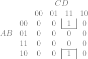
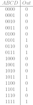
is the number that represents our lookup table. k_0 and k_1 are the values that we modulus x against to get our desired outputs out.

It looks as if we have two equations and three unknowns – which would be unsolvable – but in reality, x is the only unknown. The k values can be whatever values it takes to make the equations true.

I wrote a blog post on how to solve equations like these in a previous post: Solving Simultaneous Congruences (Chinese Remainder Theorem).

You can also use this chinese remainder theorem calculator, which is handy: Chinese Remainder Theorem Calculator

The short answer here is that the k values can be ANY numbers, so long as they are pairwise co-prime to each other – AKA they have a greatest common divisor of 1.

If we pick 3 and 4 for k0 and k1, then using the chinese remainder theorem we find that x can equal 9 and the equations are true. Technically the answer is 9 mod 12, so 21, 33, 45 and many other numbers are also valid values of x, but we are going to use the smallest answer to keep things smaller, and more manageable.

So, in this case, the value representing the lookup table would be 9. If you wanted to know what value it gave as output when you plugged in the value 0, you would modulus the lookup table (9) against k0 (3) to get the output. If you wanted to know what value it gave as output when you plugged in the value 1, you would modulus the lookup table (9) against k1 (4) to get the output. The table below shows that it passes through the value in both cases like it should:

\begin{array}{c|c|c|c} \text{Input} & \text{Symbolic} & \text{Numeric} & \text{Output} \\ \hline 0 & x \% k_0 & 9 \% 3 & 0\\ 1 & x \% k_1 & 9 \% 4 & 1\\ \end{array}

1 Bit Input, 1 Bit Output: Not Gate

Let’s do something a little more interesting. Let’s make the output bit be the reverse of the input bit. The equations we’ll want to solve are this:

x \% k_0 = 1 \\ x \% k_1 = 0

We can use 3 and 4 for k0 and k1 again if we want to. Using the Chinese remainder theorem to solve the equations gives us a value of 4 for x. Check the truth table below to see how this works:

\begin{array}{c|c|c|c} \text{Input} & \text{Symbolic} & \text{Numeric} & \text{Output} \\ \hline 0 & x \% k_0 & 4 \% 3 & 1\\ 1 & x \% k_1 & 4 \% 4 & 0\\ \end{array}

1 Bit Input, 1 Bit Output: Output Always 1

What if we wanted the output bit to always be 1 regardless of input bit?

x \% k_0 = 1 \\ x \% k_1 = 1

Using 3 and 4 for our k values again, we solve and get a value of 1 for x. Check the truth table to see it working below:

\begin{array}{c|c|c|c} \text{Input} & \text{Symbolic} & \text{Numeric} & \text{Output} \\ \hline 0 & x \% k_0 & 1 \% 3 & 1\\ 1 & x \% k_1 & 1 \% 4 & 1\\ \end{array}

Hopefully one bit input to one bit output makes sense now. Let’s move on (:

2 Bit Input, 1 Bit Output: XOR Gate

Things get a little more interesting when we bump the number of input bits up to 2. If we want to make a number which represents XOR, we now have 4 equations to solve.

x \% k_{00} = 0 \\ x \% k_{01} = 1 \\ x \% k_{10} = 1 \\ x \% k_{11} = 0

In general we will have 2^N 
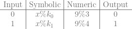
equations, where N is the number of input bits.

You might have noticed that I use subscripts for k corresponding to the input bits that the key represents. This is a convention I’ve found useful when working with this stuff. Makes it much easier to see what’s going on.

Now with four equations, we need 4 pairwise coprime numbers – no number has a common factor with another number besides 1.

Let’s pull them out of the air. Umm… 3, 4, 5, 7

Not too hard with only two bits of input, but you can see how adding input bits makes things a bit more complex. If you wanted to make something that took in two 16 bit numbers as input for example, you would need 2^32 co-prime numbers, since there was a total of 32 bits of input!

When we solve those four equations, we get a value of 21 for x.

Notice how x is larger now that we have more input bits? That is another added complexity as you add more input bits. The number representing your program can get very, very large, and require you to use “multi precision integer” math libraries to store and decode the programs, when the numbers get larger than what can be held in a 64 bit int.

Boost has a decent library for this, check out boost::multiprecision::cpp_int, it’s what I use. You can download boost from here: http://www.boost.org/doc/libs/1_59_0/more/getting_started/windows.html

Anyhow, let’s check the truth table to see if our values work:

\begin{array}{c|c|c|c} \text{Input} & \text{Symbolic} & \text{Numeric} & \text{Output} \\ \hline 00 & x \% k_{00} & 21 \% 3 & 0 \\ 01 & x \% k_{01} & 21 \% 4 & 1 \\ 10 & x \% k_{10} & 21 \% 5 & 1 \\ 11 & x \% k_{11} & 21 \% 7 & 0 \end{array}

Woot, it worked.

2 Bit Input, 2 Bit Output: OR, AND

What happens when we add another bit of output? Basically we just treat each output bit as it’s own lookup table. This means that if we have two output bits, we will have two numbers representing our program (one for each bit), and that this is true regardless of how many input bits we have.

Let’s make the left output bit (x_0 ) be the OR of the input bits and the right output bit (x_1 ) be the AND of the input bits.

That give us these two sets of equations to solve:

x_0 \% k_{00} = 0 \\ x_0 \% k_{01} = 1 \\ x_0 \% k_{10} = 1 \\ x_0 \% k_{11} = 1 \\ \\ x_1 \% k_{00} = 0 \\ x_1 \% k_{01} = 0 \\ x_1 \% k_{10} = 0 \\ x_1 \% k_{11} = 1 \\

We can use the same coprime numbers for our k values as we used in the last section (3,4,5,7). Note that we use the same k values in each set of equations. This is intentional and required for things to work out!

If we solve each set of equations we get 141 for x0, and 120 for x1.

Let’s see if that worked:

\begin{array}{c|c|c|c} \text{Input} & \text{Symbolic} & \text{Numeric} & \text{Output} \\ \hline 00 & x_0 \% k_{00}, x_1 \% k_{00} & 141 \% 3, 120 \% 3 & 00 \\ 01 & x_0 \% k_{01}, x_1 \% k_{01} & 141 \% 4, 120 \% 4 & 10 \\ 10 & x_0 \% k_{10}, x_1 \% k_{10} & 141 \% 5, 120 \% 5 & 10 \\ 11 & x_0 \% k_{11}, x_1 \% k_{11} & 141 \% 7, 120 \% 7 & 11 \end{array}

Hey, it worked again. Neat!

Example Code

Now that we have the basics worked out, here is some sample code.

The lookup table takes in 8 bits as input, mapping 0..255 to 0…2pi and gives the sine of that value as output in a float. So it has 8 bits of input and 32 bits of output.

#include <vector>
#include <boost/multiprecision/cpp_int.hpp>
#include <stdint.h>
#include <string.h>
#include <memory>

typedef boost::multiprecision::cpp_int TINT;
typedef std::vector<TINT> TINTVec;

const float c_pi = 3.14159265359f;

//=================================================================================
void WaitForEnter ()
{
    printf("nPress Enter to quit");
    fflush(stdin);
    getchar();
}

//=================================================================================
static TINT ExtendedEuclidianAlgorithm (TINT smaller, TINT larger, TINT &s, TINT &t)
{
    // make sure A <= B before starting
    bool swapped = false;
    if (larger < smaller)
    {
        swapped = true;
        std::swap(smaller, larger);
    }

    // set up our storage for the loop.  We only need the last two values so will
    // just use a 2 entry circular buffer for each data item
    std::array<TINT, 2> remainders = { larger, smaller };
    std::array<TINT, 2> ss = { 1, 0 };
    std::array<TINT, 2> ts = { 0, 1 };
    size_t indexNeg2 = 0;
    size_t indexNeg1 = 1;

    // loop
    while (1)
    {
        // calculate our new quotient and remainder
        TINT newQuotient = remainders[indexNeg2] / remainders[indexNeg1];
        TINT newRemainder = remainders[indexNeg2] - newQuotient * remainders[indexNeg1];

        // if our remainder is zero we are done.
        if (newRemainder == 0)
        {
            // return our s and t values as well as the quotient as the GCD
            s = ss[indexNeg1];
            t = ts[indexNeg1];
            if (swapped)
                std::swap(s, t);

            // if t < 0, add the modulus divisor to it, to make it positive
            if (t < 0)
                t += smaller;
            return remainders[indexNeg1];
        }

        // calculate this round's s and t
        TINT newS = ss[indexNeg2] - newQuotient * ss[indexNeg1];
        TINT newT = ts[indexNeg2] - newQuotient * ts[indexNeg1];

        // store our values for the next iteration
        remainders[indexNeg2] = newRemainder;
        ss[indexNeg2] = newS;
        ts[indexNeg2] = newT;

        // move to the next iteration
        std::swap(indexNeg1, indexNeg2);
    }
}

//=================================================================================
void MakeKey (TINTVec &keys, TINT &keysLCM, size_t index)
{
    // if this is the first key, use 3
    if (index == 0)
    {
        keys[index] = 3;
        keysLCM = keys[index];
        return;
    }

    // Else start at the last number and keep checking odd numbers beyond that
    // until you find one that is co-prime.
    TINT nextNumber = keys[index - 1];
    while (1)
    {
        nextNumber += 2;
        if (std::all_of(
            keys.begin(),
            keys.begin() + index,
            [&nextNumber] (const TINT& v) -> bool
            {
                TINT s, t;
                return ExtendedEuclidianAlgorithm(v, nextNumber, s, t) == 1;
            }))
        {
            keys[index] = nextNumber;
            keysLCM *= nextNumber;
            return;
        }
    }
}

//=================================================================================
void CalculateLookupTable (
    TINT &lut,
    const std::vector<uint64_t> &output,
    const TINTVec &keys,
    const TINT &keysLCM,
    const TINTVec &coefficients,
    size_t bitMask
)
{
    // figure out how much to multiply each coefficient by to make it have the specified modulus residue (remainder)
    lut = 0;
    for (size_t i = 0, c = keys.size(); i < c; ++i)
    {
        // we either want this term to be 0 or 1 mod the key.  if zero, we can multiply by zero, and
        // not add anything into the bit value!
        if ((output[i] & bitMask) == 0)
            continue;

        // if 1, use chinese remainder theorem
        TINT s, t;
        ExtendedEuclidianAlgorithm(coefficients[i], keys[i], s, t);
        lut = (lut + ((coefficients[i] * t) % keysLCM)) % keysLCM;
    }
}

//=================================================================================
template <typename TINPUT, typename TOUTPUT, typename LAMBDA>
void MakeModulus (TINTVec &luts, TINTVec &keys, LAMBDA &lambda)
{
    // to keep things simple, input sizes are being constrained.
    // Do this in x64 instead of win32 to make size_t 8 bytes instead of 4
    static_assert(sizeof(TINPUT) < sizeof(size_t), "Input too large");
    static_assert(sizeof(TOUTPUT) < sizeof(uint64_t), "Output too large");

    // calculate some constants
    const size_t c_numInputBits = sizeof(TINPUT) * 8;
    const size_t c_numInputValues = 1 << c_numInputBits;
    const size_t c_numOutputBits = sizeof(TOUTPUT) * 8;

    // Generate the keys (coprimes)
    TINT keysLCM;
    keys.resize(c_numInputValues);
    for (size_t index = 0; index < c_numInputValues; ++index)
        MakeKey(keys, keysLCM, index);

    // calculate co-efficients for use in the chinese remainder theorem
    TINTVec coefficients;
    coefficients.resize(c_numInputValues);
    fill(coefficients.begin(), coefficients.end(), 1);
    for (size_t i = 0; i < c_numInputValues; ++i)
    {
        for (size_t j = 0; j < c_numInputValues; ++j)
        {
            if (i != j)
                coefficients[i] *= keys[j];
        }
    }

    // gather all the input to output mappings by permuting the input space
    // and storing the output for each input index
    std::vector<uint64_t> output;
    output.resize(c_numInputValues);
    union
    {
        TINPUT value;
        size_t index;
    } input;
    union
    {
        TOUTPUT value;
        size_t index;
    } outputConverter;

    for (input.index = 0; input.index < c_numInputValues; ++input.index)
    {
        outputConverter.value = lambda(input.value);
        output[input.index] = outputConverter.index;
    }

    // iterate through each possible output bit, since each bit is it's own lut
    luts.resize(c_numOutputBits);
    for (size_t i = 0; i < c_numOutputBits; ++i)
    {
        const size_t bitMask = 1 << i;
        CalculateLookupTable(
            luts[i],
            output,
            keys,
            keysLCM,
            coefficients,
            bitMask
        );
    }
}

//=================================================================================
int main (int argc, char **argv)
{
    // Look up tables encodes each bit, keys is used to decode each bit for specific
    // input values.
    TINTVec luts;
    TINTVec keys;

    // this is the function that it turns into modulus work
    typedef uint8_t TINPUT;
    typedef float TOUTPUT;
    auto lambda = [] (TINPUT input) -> TOUTPUT
    {
        return sin(((TOUTPUT)input) / 255.0f * 2.0f * c_pi);
    };

    MakeModulus<TINPUT, TOUTPUT>(luts, keys, lambda);

    // show last lut and key to show what kind of numbers they are
    std::cout << "Last Lut: " << *luts.rbegin() << "n";
    std::cout << "Last Key: " << *keys.rbegin() << "n";

    // Decode all input values
    std::cout << "n" << sizeof(TINPUT) << " bytes input, " << sizeof(TOUTPUT) << " bytes outputn";
    for (size_t keyIndex = 0, keyCount = keys.size(); keyIndex < keyCount; ++keyIndex)
    {
        union
        {
            TOUTPUT value;
            size_t index;
        } result;

        result.index = 0;

        for (size_t lutIndex = 0, lutCount = luts.size(); lutIndex < lutCount; ++lutIndex)
        {
            TINT remainder = luts[lutIndex] % keys[keyIndex];
            size_t remainderSizeT = size_t(remainder);
            result.index += (remainderSizeT << lutIndex);
        }

        TINT remainder = luts[0] % keys[keyIndex];
        std::cout << "i:" << keyIndex << " o:" << result.value << "n";
    }

    WaitForEnter();
    return 0;
}

Here is some output from the program. The first is to show what the last (largest) look up table and key look like. Notice how large the look up table number is!

Here it shows some sine values output from the program, using modulus against the large numbers calculated, to get the bits of the result out:

How to Get Lots of Pairwise Co-Prime Numbers?

You can generate a list of pairwise coprimes using brute force. Have an integer that you increment, and check if it’s pairwise co-prime to the existing items in the list. If it is, add it to the list! Rinse and repeat until you have as many as you want.

That is the most practical way to do it, but there are two other interesting ways I wanted to mention.

The first way is using Fermat numbers. The Fermat numbers are an infinite list of pairwise co-prime numbers and are calculated as 2^{2^n}+1 where n is an integer. Fermat numbers also have the benefit that you can get the nth item in the list without calculating the numbers that came before it. The only problem is that the numbers grow super huge very fast. The first 7 values are: 3, 5, 17, 257, 65537, 4294967297, 18446744073709551617. If Fermat numbers didn’t grow so quickly, they sure would be useful for things like this technique.

The second way is using something called Sylvester’s sequence. It too is an infinite list of pairwise co-prime numbers, and it too grows very large very quickly unfortunately. I also don’t believe there is a way to calculate the Nth item in the list directly. Every number is based on previous numbers, so you have to calculate them all from the beginning. No random access!

Beyond Binary

In this post I showed how to work in binary digits, but there is no reason why you have to encode single bits in the lookup tables.

Instead of encoding 0 or 1 in each modulus “lookup table”, you could also perhaps store base 10 numbers in the tables and have 0-9. Or, maybe you encode a byte per lookup table.

Encoding more than one bit effectively makes both your input and your output smaller, which helps the algorithm do more with less.

Your keys will need to be larger though, since the keys have to be larger than the value you plan to store, and your resulting lookup table will be a larger number as well. It might make the technique more worth while though.

I’ll leave that as an exercise for you. If try it and find neat stuff, post a comment and let us know, or drop me an email or something. It’d be neat to hear if people find any practical usage cases of this technique 😛

The End, For Now!

I want to point out that increasing the number of input bits in this technique is a pretty expensive thing to do, but increasing the number of output bits is a lot cheaper. It kind of makes sense in a way if you think about it. Input bits add information from the outside world that must be dealt with, while output bits are just fluff that can easily be diluted or concentrated by adding or removing bits that are associated with, and calculated from, the input bits.

Another problem you may have noticed with this technique is that if you have a really expensive calculation that you are trying to “flatten” into modulus math like this, that you have to run that calculation many, many times to know what values a lookup table would give you. You have to run it once per possible input to get every possible output. That is expected when making a lookup table, since you are paying a cost up front to make things faster later.

The paper I’m working on changes things a bit though. One of the things it does is it makes it so doing this technique only requires that you evaluate the function once, and it calculates all values simultaneously to give the end result that you can then do modulus against. It’s pretty cool IMO and I will share more details here as soon as I am able – and yes, i have actual working code that does that, believe it or not! I’m looking forward to being able to share it later on. Maybe someone will find some really cool usage case for it.