In the last post, I talked about imaginary numbers, complex numbers, and how to use them to rotate vectors in 2d.
In this post, I want to share another interesting type of number called a “Dual Number” that uses the symbol ε (epsilon) and has a neat trick of automatically calculating the derivative of a function while you calculate the value of the function at the same time.
Dual numbers are pretty similar to imaginary numbers but there is one important difference. With imaginary numbers, i^2 = -1, but with dual numbers, ε^2 = 0 (and ε is not 0!). That may seem like a small difference, but oddly, that opens up a whole interesting world of mathematical usefulness.
Before we dig into automatic differentiation, I want to go over the mathematical basics for how dual numbers behave.
Basic Dual Number Math
Adding dual numbers is the same as adding complex numbers; you just add the real and dual parts separately:
(3 + 4ε) + (1 + 2ε) = 4 + 6ε
Subtraction works the same way as well:
(3 + 4ε) – (1 + 2ε) = 2 + 2ε
To multiply dual numbers, you use F.O.I.L. just like you do with complex numbers:
(3 + 4ε) * (1 + 2ε) =
3 + 6ε + 4ε + 8ε^2 =
3 + 10ε + 8ε^2
However, since ε^2 is zero, the last term 8ε^2 disappears:
3 + 10ε
It’s interesting to note that with complex numbers, the i^2 became -1, so the last term changed from imaginary to real, meaning that the imaginary numbers fed back into the real numbers during multiplication. With dual numbers, that isn’t the case, the dual numbers don’t feed back into the real numbers during multiplication.
In both complex and dual numbers the real terms do affect the non real terms during multiplication.
The division operator relates to the conjugate. I have source code for it below, and some of the links at the end of the post go into the details of that and other operations.
Quick Review: Derivatives (Slope)
If you know the line formula y=mx+b, but you don’t know what a derivative is you are in luck. Remember how “m” is the slope of the line, specifying how steep it is? That is what the derivative is too, it’s just the slope.
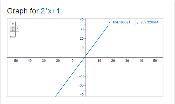
Below is a graph of y=2x+1. At every point on that line, the derivative (or slope) is 2. That means that for every step we make on the x axis to the right (positive direction), we make 2 steps up on the y axis (positive direction).
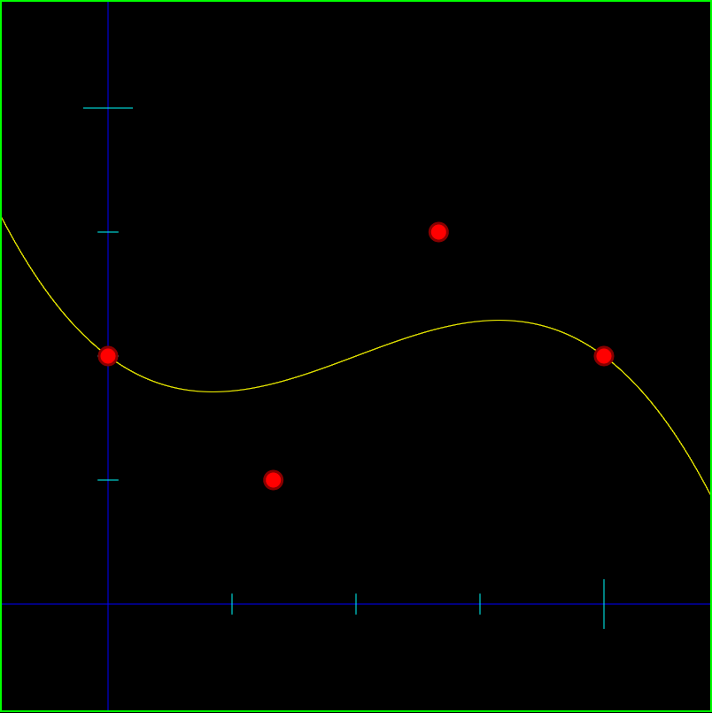
Now, check out this graph of y=x^2-0.2
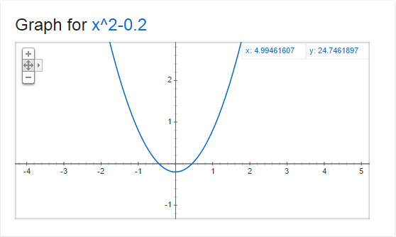
The derivative (or slope) at every point on this graph is 2x. That means that the slope changes depending on where the x coordinate is!
So, when x=0, the slope is 0. You can see that in the graph where x=0, that it is horizontal, meaning that a step on the x axis becomes no steps on the y axis (only at that point where x is 0, and only if you take an infinitely small step).
When x is 1, the slope is 2, when x is 2, the slope is 4, when x is 3, the slope is 6. Since the numbers increase as we increase x from 0, that tells us that the graph gets steeper as we go to the right, which you can see in the graph.
Alternately, when x is -1, the slope is -2, when x is -2, the slope is -4, and when x is -3, the slope is -6. This shows us that as we decrease x from 0, the graph gets steeper in the opposite direction, which you can see in the graph as well.
What is Automatic Differentiation?
Let’s say you have a function (possibly a curve) describing the path of a rocket, and you want to make the rocket point down the path that it’s traveling.
One way you might do this is to evaluate your function f(T) to get the current location of your rocket (where T is how long the rocket has been flying), and then calculate the derivative f'(T) to find the slope of the graph at that point so that you can orient the rocket in that direction.
You could calculate the value and slope of the function at time T independently easily enough if you know how to get the derivative of a function (a calculus topic), or use wolframalpha.com.
However, if you have a complex equation, or maybe if the equation is controlled by user input, or game data, it might not be so easy to figure out what the derivative is at run time.
For instance… imagine having a function that rolled random numbers to figure out what mathematical operation it should preform on a number next (if we roll a 0, add 3, if we roll a 1 multiply by 2, if we roll a 2, square the number… etc). It isn’t going to be simple to take the derivative of the same mathematical function.
Here enters automatic differentiation (or AD). AD lets you calculate the derivative WHILE you are calculating the value of the function.
That way, you can do whatever math operations you want on your number, and in the end you will have both the value of f(T) as well as the derivative f'(T).
Using ε for Automatic Differentiation
You can use dual number operations on numbers to calculate the value of f(x) while also calculating f'(x) at the same time. I’ll show you how with a simple example using addition and multiplication like we went over above.
We’ll start with the function f(x)=3x+2, and calculate f(4) and f'(4).
the first thing we do is convert our 4 into a dual number, using 1 for the dual component, since we are plugging it in for the value of x, which has a derivative of 1.
4+1ε
Next, we want to multiply that by the constant 3, using 0 for the dual component since it is just a constant (and the derivative of a constant is 0)
(4+1ε) * (3 + 0ε) =
12 + 0ε + 3ε + 0ε^2 =
12 + 3e
Lastly, we need to add the constant 2, using 0 again for the dual component since it’s just a constant.
(12 + 3ε) + (2 + 0ε) =
14 + 3ε
In our result, the real number component (14) is the value of f(4) and the dual component (3) is the derivative f'(4), which is correct if you work it out!
Let’s try f(5). First we convert 5 to a dual number, with the dual component being 1.
5 + 1ε
Next we need to multiply it by the constant 3 (which has a dual component of 0)
(5 + 1ε) * (3 + 0e) =
15 + 0ε + 3ε + 0ε^2 =
15 + 3ε
Now, we add the constant 2 (which has a dual component of 0 again since it’s just a constant)
(15 + 3ε) + (2 + 0ε) =
17 + 3ε
So, our answer says that f(5) = 17, and f'(5) = 3, which again you can verify is true!
Quadratic Example
The example above worked well but it was a linear function. What if we want to do a function like f(x) = 5x^2 + 4x + 1?
Let’s calculate f(2). We are going to first calculate the 5x^2 term, so we need to start by making a dual number for the function parameter x:
(2 + 1ε)
Next, we need to multiply it by itself to make x^2:
(2 + 1ε) * (2 + 1ε) =
4 + 2ε + 2ε + 1ε^2 =
4 + 4ε
(remember that ε^2 is 0, so the last term disappears)
next, we multiply that by the constant 5 to finish making the 5x^2 term:
(4 + 4ε) * (5 + 0ε) =
20 + 0ε + 20ε + 0ε^2 =
20 + 20ε
Now, putting that number aside for a second we need to calculate the “4x” term by multiplying the value we plugged in for x by the constant 4
(2 + 1ε) * (4 + 0ε) =
8 + 0ε + 4ε + 0ε^2 =
8 + 4ε
Next, we need to add the last 2 values together (the 5x^2 term and the 4x term):
(20 + 20ε) + (8 + 4ε) =
28 + 24ε
Lastly, we need to add in the last term, the constant 1
(28 + 24ε) + (1 + 0ε) =
29 + 24e
There is our answer! For the equation y = 5x^2 + 4x + 1, f(2) = 29 and f'(2) = 24. Check it, it’s correct (:
As one last example let’s calculate f(10) and f'(10) with the same function above y = 5x^2 + 4x + 1.
First, to start calculating the 5x^2 term, we need to make 10 into a dual number and multiply it by itself to make x^2:
(10 + 1ε) * (10 + 1ε) =
100 + 10ε + 10ε + 1ε^2 =
100 + 20ε
Next, we multiply by the constant 5 to finish making the 5x^2 term:
(100 + 20ε) * (5 + 0ε) =
500 + 0ε + 100ε + 0ε^2 =
500 + 100ε
Putting that aside, let’s calculate the 4x term by multiplying our x value by the constant 4:
(10 + 1ε) * (4 + 0ε) =
40 + 0ε + 4ε + 0ε^2 =
40 + 4ε
Lastly, let’s add our terms: 5x^2, 4x and the constant 1
(500 + 100ε) + (40 + 4ε) + (1 + 0ε) =
541 + 104ε
The answer tells us that for the equation y = 5x^2 + 4x + 1, f(10) = 541 and f'(10) = 104.
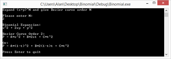
Sample Code
There are lots of other mathematical operations that you can do with dual numbers. I’ve collected as many as I was able to find and made up some sample code that uses them. The sample code is below, as well as the program output.
#include
#include
#define PI 3.14159265359f
// In production code, this class should probably take a template parameter for
// it's scalar type instead of hard coding to float
class CDualNumber
{
public:
CDualNumber (float real = 0.0f, float dual = 0.0f)
: m_real(real)
, m_dual(dual)
{
}
float Real () const { return m_real; }
float Dual () const { return m_dual; }
private:
float m_real;
float m_dual;
};
//----------------------------------------------------------------------
// Math Operations
//----------------------------------------------------------------------
inline CDualNumber operator + (const CDualNumber &a, const CDualNumber &b)
{
return CDualNumber(a.Real() + b.Real(), a.Dual() + b.Dual());
}
inline CDualNumber operator - (const CDualNumber &a, const CDualNumber &b)
{
return CDualNumber(a.Real() - b.Real(), a.Dual() - b.Dual());
}
inline CDualNumber operator * (const CDualNumber &a, const CDualNumber &b)
{
return CDualNumber(
a.Real() * b.Real(),
a.Real() * b.Dual() + a.Dual() * b.Real()
);
}
inline CDualNumber operator / (const CDualNumber &a, const CDualNumber &b)
{
return CDualNumber(
a.Real() / b.Real(),
(a.Dual() * b.Real() - a.Real() * b.Dual()) / (b.Real() * b.Real())
);
}
inline CDualNumber sqrt (const CDualNumber &a)
{
float sqrtReal = ::sqrt(a.Real());
return CDualNumber(
sqrtReal,
0.5f * a.Dual() / sqrtReal
);
}
inline CDualNumber pow (const CDualNumber &a, float y)
{
return CDualNumber(
::pow(a.Real(), y),
y * a.Dual() * ::pow(a.Real(), y - 1.0f)
);
}
inline CDualNumber sin (const CDualNumber &a)
{
return CDualNumber(
::sin(a.Real()),
a.Dual() * ::cos(a.Real())
);
}
inline CDualNumber cos (const CDualNumber &a)
{
return CDualNumber(
::cos(a.Real()),
-a.Dual() * ::sin(a.Real())
);
}
inline CDualNumber tan (const CDualNumber &a)
{
return CDualNumber(
::tan(a.Real()),
a.Dual() / (::cos(a.Real()) * ::cos(a.Real()))
);
}
inline CDualNumber atan (const CDualNumber &a)
{
return CDualNumber(
::atan(a.Real()),
a.Dual() / (1.0f + a.Real() * a.Real())
);
}
inline CDualNumber SmoothStep (CDualNumber x)
{
// f(x) = 3x^2 - 2x^3
// f'(x) = 6x - 6x^2
return x * x * (CDualNumber(3) - CDualNumber(2) * x);
}
//----------------------------------------------------------------------
// Test Functions
//----------------------------------------------------------------------
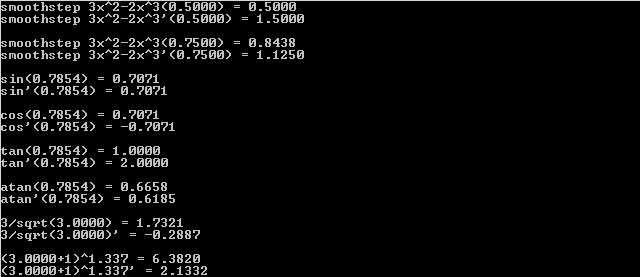
void TestSmoothStep (float x)
{
CDualNumber y = SmoothStep(CDualNumber(x, 1.0f));
printf("smoothstep 3x^2-2x^3(%0.4f) = %0.4fn", x, y.Real());
printf("smoothstep 3x^2-2x^3'(%0.4f) = %0.4fnn", x, y.Dual());
}
void TestTrig (float x)
{
CDualNumber y = sin(CDualNumber(x, 1.0f));
printf("sin(%0.4f) = %0.4fn", x, y.Real());
printf("sin'(%0.4f) = %0.4fnn", x, y.Dual());
y = cos(CDualNumber(x, 1.0f));
printf("cos(%0.4f) = %0.4fn", x, y.Real());
printf("cos'(%0.4f) = %0.4fnn", x, y.Dual());
y = tan(CDualNumber(x, 1.0f));
printf("tan(%0.4f) = %0.4fn", x, y.Real());
printf("tan'(%0.4f) = %0.4fnn", x, y.Dual());
y = atan(CDualNumber(x, 1.0f));
printf("atan(%0.4f) = %0.4fn", x, y.Real());
printf("atan'(%0.4f) = %0.4fnn", x, y.Dual());
}
void TestSimple (float x)
{
CDualNumber y = CDualNumber(3.0f) / sqrt(CDualNumber(x, 1.0f));
printf("3/sqrt(%0.4f) = %0.4fn", x, y.Real());
printf("3/sqrt(%0.4f)' = %0.4fnn", x, y.Dual());
y = pow(CDualNumber(x, 1.0f) + CDualNumber(1.0f), 1.337f);
printf("(%0.4f+1)^1.337 = %0.4fn", x, y.Real());
printf("(%0.4f+1)^1.337' = %0.4fnn", x, y.Dual());
}
int main (int argc, char **argv)
{
TestSmoothStep(0.5f);
TestSmoothStep(0.75f);
TestTrig(PI * 0.25f);
TestSimple(3.0f);
return 0;
}
Here is the program output:
Closing Info
When you are thinking what number ε has to be so that ε^2 is 0 but ε is not 0, you may be tempted to think that it is an imaginary number, just like i (the square root of -1) that doesn’t actually exist. This is actually not how it is… I’ve seen ε described in two ways.
One way I’ve seen it described is that it’s an infinitesimal number. That sort of makes sense to me, but not in a concrete and tangible way.
The way that makes more sense to me is to describe it as a matrix like this:
[0, 1]
[0, 0]
If you multiply that matrix by itself, you will get zero(s) as a result.
In fact, an alternate way to implement the dual numbers is to treat them like a matrix like that.
I also wanted to mention that it’s possible to modify this technique to get the 2nd derivative of a function or the 3rd, or the Nth. It isn’t only limited to the 1st derivative. Check the links at the bottom of this post for more info, but essentially, if you want 1st and 2nd derivative, you need to make it so that ε^3 = 0 instead of ε^2 = 0. There is a way to do that with matrices.
Another neat thing is that you can also extend this into multiple dimensions. This is useful for situations like if you have some terrain described by mathematical functions, when you are walking the grid of terrain to make vertex information, you can get the slope / gradient / surface normal at the same time.
Lastly, I wanted to mention a different kind of number called a hyperbolic number.
The imaginary number i^2 = -1 and we can use it to do 2d rotations.
The dual number ε^2 is 0 (and ε is not 0) and we can use it to do automatic differentiation.
Hyperbolic numbers have j, and j^2 = 1 (and j is not 1). I’m not sure, but I bet they have some interesting usefulness to them too. It would be interesting to research that more sometime. If you know anything about them, please post a comment!
Links
This shadertoy is what got me started looking into dual numbers. It’s a mandelbrot viewer done by iq using dual numbers to estimate a distance from a point to the mandelbrot set (as far as I understand it anyhow, ha!). He uses that estimated distance to color the pixels.
Shadertoy: Dual Complex Numbers
I didn’t get very much into the reasons of why this works (has to do with taylor series terms disappearing if ε^2 is 0), or the rigorous math behind deriving the operators, but here are some great links I found researching this stuff and putting this blog post together.
Wikipedia: Dual Number
[Book] Dual-Number Methods in Kinematics, Statics and Dynamics By Ian Fischer
[GDC2012] Math for Game Programmers: Dual Numbers by Gino van den Bergen
Stackexchange: Implementing trig functions for dual numbers
Exact numeric nth derivatives
Automatic Differentiation with Dual numbers
Wikipedia: Automatic Differentiation


 for ANY value
  using the binomial theorem (well, N has to be a positive integer…)


 case. The next row down is “1,2,1” which is the constants multiplied by each term for the
  case. Lastly the next row down (fourth row) is “1,3,3,1” which is the constants multiplied by each term for the
  case. Essentially, you just use the
  th tow of pascals triangle to come up with the constants to multiply each term by.
 , and then multiply each term by a unique control point (A,B,C,etc). After you have your equation, you can optionally replace all
  ‘s with
  , or you can just remember that when you evaluate the equation, since the first form is less messy.


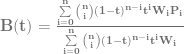
 (Sigma, going from 0 to n) means that you are going to sum (add) together n+1 terms (it includes both 0 and n), using i as the loop variable in your summation. It’s basically a for loop, adding together each iteration of the for loop. Everything that comes after is what happens during each iteration of the for loop that gets summed together.
 part means to take the ith number from the (n+1)th row of Pascal’s triangle. More formally, this specifies to use specific binomial coefficients.
 means that you multiply the binomial coefficient by s to the (n-i)th power, and t to the ith power. This is the same as saying s starts at power n and counts down left to right, while t starts at 0 and counts up left to right. This fits the pattern we saw above in binomial expansion.
 which means to use the ith P. So, P is basically an array with n+1 elements. This array is the control points, so each P is a different control point.