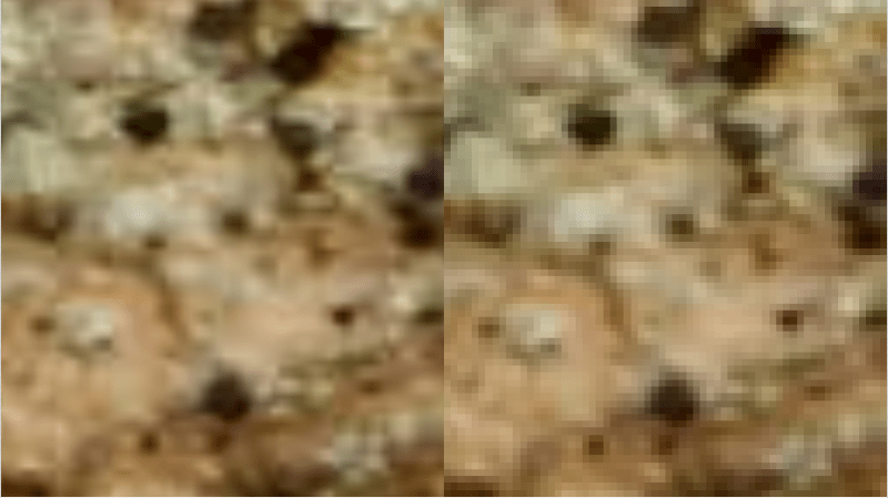
This is the last of my planned posts on probabilistic algorithms. There may be more in the future, but the initial volley is finished 😛
Thanks again to Ben Deane for exposure to this really interesting area of computer science.
This post is about HyperLogLog, which is used to estimate a count of how many “uniques” there are in a stream of data. It can also do intersection and union between two hyperloglog objects allowing you to see how many items HLL objects have in common. It was invented in 2007 and is currently used in many big data situations including use by Google and Redis and Amazon.
This algorithm is probabilistic in that you can trade storage space for accuracy. You can calculate how much accuracy to expect for a given amount of storage, or calculate how much storage you’d need for a specific amount of accuracy.
If this sounds a lot like the first probabilistic algorithm post I made (Estimating Counts of Distinct Values with KMV) that means you have been paying attention. HyperLogLog is in the same family of algorithms, but it is way better at most things than KMV is, and seems to be the current standard for DV Sketches (distinct value estimators). The one thing KMV seems to be better at is calculating intersections between objects, which i’ll talk about more below.
To give you an idea of the power of HyperLogLog, here’s a quote from the paper it was first described in (link at end of post):
“…the new algorithm makes it possible to estimate cardinalities well beyond 10^9 with a typical accuracy of 2% while using a memory of only 1.5 kilobytes”
By the end of this post you should understand how that is possible, and also be able to start with the sample code and have HyperLogLog capabilities in your own C++ project immediately!
A Usage Case: Upvoting
A usage case for this algorithm would be adding an “upvote” button to a webpage.
A naive solution to this would be to have an upvote button that when clicked would increment a counter on the server. That is problematic though because people can vote as many times as they want. You could hack together a solution to this by having some client side cookies and javascript limiting people from doing that, but all your security is out the window since it’s a client side fix, and you will soon have trolls spamming your vote counters by doing raw HTTP requests to your servers, to ruin your day, just because they can.
A less naive solution would be to have some unique identifier per user – whether that was something like a username, or just an IP address – and store that in a voting table, only allowing the counter to increment if the person wasn’t already in the table, and entering them into the table when doing the increment.
The problem with that solution is that the table of users who have already voted might get extremely huge, causing lots of memory usage to hold it, lots of processing time to see if a user exists in the table already (even with a hash based lookup), and it doesn’t parallelize very well to multiple servers. You also have to implement some protection against race conditions around the “look for user in table, increment vote counter, add user to table” work, which means some potentially costly synchronization logic.
A better solution would be to use HyperLogLog and Here are some reasons why:
- It has a fixed size you determine in advance. The bold quote from the paper would indicate that 1.5KB is likely enough for our needs, being able to count over one billion unique values. Bringing it up to 2KB would be enough to store a heck of a lot more, like somewhere up near 2^250 unique items.
- It automatically disallows the same item being accounted for more than once, so our multiple votes from same voter problem is gone with no need for costly synchronization work.
- It lends itself well to being parallelized across machines, or just using SIMD / GPGPU if you wanted to squeeze some more performance out of it.
- You can very quickly do set operations on multiple HLL objects.
The first three items solve the problems in the naive solutions, but the fourth adds some bonus functionality that is pretty cool.
Using set operations, you can do things like figure out if the same people are upvoting a dulce de leche flan desert compared to a cheesy grits recipe, and you can calculate that VERY QUICKLY.
A possibly naive way to suggest a recipe to a user would be to show them recipes that a lot of people have upvoted.
A more custom tailored suggestion (and thus, hopefully a better suggestion) would be when a person votes on a recipe, you can tell them “hey, a lot of the same people that upvoted the recipe you just upvoted also upvoted this other recipe, why don’t you check it out!”
So now, you don’t just have a voting system, you now also have a CLASSIFICATION SYSTEM.
Yeah ok, so that’s a little hand wavy and making a real suggestion system has more details to solve than just those etc etc, but hopefully you can see how this algorithm can be a fundamental building block to many “big data” problems.
Onto the details of how it works!
Basic Premise – Coin Flips
When you flip a coin, what are the odds that it will be heads? There’s even chance of heads or tails, so the chance of a heads is 1 in 2 or 1/2 or 50%.
What are the odds that if you flip a coin twice it a row it will be heads both times? Well, on each flip there is a 50% chance, so you multiply .5 * .5 to get the answer which is .25 or 25%. There’s a 25% chance, or a 1 in 4 chance, that you will flip heads twice in a row with two coin flips. It’s the same chance that you will flip two tails in a row, or that you will flip heads then tails, or tails then heads. All possible outcomes have the same probability.
Another way to look at this, instead of probability, is to see how many combinations possible there are like this:
| Sequence Number |
Sequence |
| 0 |
heads, heads |
| 1 |
heads, tails |
| 2 |
tails, heads |
| 3 |
tails, tails |
There’s a 100% chance that two coin flips will be somewhere in those four results, and all results have an even chance of happening, so result 0 “heads, heads” has a 1 in 4 chance of happening. All of the results above have a 1 in 4 chance. Interestingly, looking at the above table you can also see that there is a 2/4 chance that the first flip will be heads, which is also 1/2, 1 in 2 or 50% chance. That agrees with what we said before, that if only doing one coin flip (the first coin flip), there is a 50% chance of heads or tails.
If you switched to 3 coin flips, there would be a 1 in 8 chance of any specific event happening, since there are 8 possible outcomes:
| Sequence Number |
Sequence |
| 0 |
heads, heads, heads |
| 1 |
heads, heads, tails |
| 2 |
heads, tails, heads |
| 3 |
heads, tails, tails |
| 4 |
tails, heads, heads |
| 5 |
tails, heads, tails |
| 6 |
tails, tails, heads |
| 7 |
tails, tails, tails |
It doesn’t matter which specific sequence you are looking at above, the chance that 3 coin flips will result in any of those specific sequences is 1 in 8.
In fact, for N coin flips, the probability that you will encounter any specific sequence (permutation) of heads and tails is 1 in 2^N, or 1/(2^N).
Now, let’s change it up a bit. What are the odds that you will have some number of heads in a row, and then a tails? In other words, what are the odds that you will have a “run” of heads of a specified length?
well, a run of 0 would just be you flip the coin once and get tails. Since you are doing one coin flip and you are looking for a specific one of two possible outcomes to happen, the probability is or 1 in 2, or 1/2, or 50%.
A run of 1 would mean you flipped the coin once, got heads, flipped it again and got tails. Since you are doing two coin flips and are looking for a specific one of four possible outcomes, the probability of that happening is 1/2*1/2 = 1/4, or 1 in 4, or 25%.
A run of 2 means heads, heads, tails. 3 coin flips = 1/2*1/2*1/2 = 1/8, or 1 in 8, or 12.5%.
By now you may have noticed that the probability for getting N heads and then a tail is just 1 in the number of coin flips, and the number of coin flips is 2^(N+1).
More formally, the odds of getting N heads and then a tail is 1/(2^(N+1)).
Let’s now swap out the idea of heads and tails with the idea of binary digits 0 and 1 in a sequence of random numbers. Think of “heads” as 0, and “tails” as 1.
If you generate a random bit (binary digit), there is a 50% chance it will be a 0, and a 50% chance it will be a 1.
If you generate two random bits, there is a 25% chance for each of the possible outcomes below:
| Sequence Number |
Sequence |
| 0 |
00 |
| 1 |
01 |
| 2 |
10 |
| 3 |
11 |
Now, what are the odds that in a random binary number, we will have N zeros and then a 1?
Don’t let the binary digits scare you, it’s the same answer as the coin flip question: 1/(2^(N+1))
An interesting property of this is that if you ask for a random 8 bit binary number and get xxxxx100, using the formula above, you know there is a 1 in 8 chance that a random number would end in “100”.
Using this information you can say to yourself “i’ll bet I’ve seen about 8 different random numbers at this point”, and that’s a fairly decent guess, without actually having had to pay attention to any of the numbers that came before.
A better idea though would be to watch all the random numbers as they are generated, and keep track the longest run of zeros you’ve seen on the right side of any number.
Using this “longest run seen” value, you can guess how many unique random numbers you’ve seen so far. If the longest run you’ve seen is N zeros and then a 1, the guess as to how many random numbers you’ve seen is 2^(N+1).
If you’ve seen a maximum of 4 zeros and a 1 (xxx10000), you’ve probably seen about 32 numbers on average. If you’ve seen at maximum 2 zeros and a 1 (xxxxx100), you’ve probably seen about 8 numbers on average.
Since by definition, randomness is RANDOM, there will be fluctuation and your guess will not always be so accurate. You might have only seen one random number, but it’s value may have been 10000000 (0x80), which would incorrectly cause you to estimate that 256 items have been seen (2^8), when in fact only a single item has been seen.
To combat this, HyperLogLog uses multiple registers (counters) to keep multiple counts, and then averages the estimates together. More info on that below, but for now, hopefully you can see how that would smooth things out towards a more average case. The more registers you use, the more “average case” your estimation should be, so the more accurate your estimate should be.
There’s an interesting twist here though… you aren’t actually estimating how many random numbers you’ve seen, but instead are estimating how many UNIQUE random numbers you’ve seen. Random numbers can repeat, but this count estimation will only count each unique value once, no matter how many times it appears.
To help visualize that, no matter how many times you see 10110100 – whether it’s only once, or ten thousand times – the longest run will still be 2. After you’ve seen ten thousand of those numbers, as soon as you see the next number 10011000, the longest run will then be 3.
That may sound like a trivial difference that we are counting uniques, and not actual values, but as the next section will show, it’s actually a very important difference, and is where this technique derives it’s power.
Also, if we were counting non uniques, we could just use an integer and increment it for each item we saw (;
Hashing Functions as Pseudorandom Number Generators
An interesting property of good hashing algorithms is that the output you get when you hash an object will be indistinguishable from random numbers. If you hash 3, you’ll get a random number, and if you hash 4, you’ll likely get a completely different random number. You can’t tell from the output what the nature of the input was, or how similar the input objects were.
But, of course, when you put the same input into a hash function, you will always get the same output.
These two properties are what makes hash functions so useful in what we are trying to do in HLL.
Quick Tangent: These same properties also apply to encryption by the way. The fact that they are random output is why hashed and encrypted data doesn’t compress very well. There are no patterns in the data that can be exploited to express the data as anything shorter than the full length of data itself. You should not be able to gain any knowledge about the nature of the input by looking at the output, except perhaps the size of the source data in the case of encryption. Also, whereas hashes are not reversible at all, encryption is only reversible if you have the encryption key (password). HLL and similar algorithms use hashes, not encryption, because they want a fixed size output, and they don’t care about reversing the process.
The output of the hash function is the source of the pseudorandom numbers that we plug into the HyperLogLog algorithm, and is what allows us to count uniques of any type of thing, so long as that thing can be hashed.
So, to do HLL counting, you hash every object you see in a stream keeping track of the longest run of zeros (in binary) you’ve seen in the resulting hashes. You store “longest runs seen” in multiple registers which you can then later use to get an averaged estimate of unique items encountered. That’s all there is to it.
MAGIC!
That’s how things work from a high level, now let’s get into the nitty gritty a bit…
Handling Multiple Registers
Let’s say you have a hash function that spits out a 32 bit hash, which is a pretty common thing for HLL implementations.
We talked about figuring out the length of the run of 0’s in the hash output, but if you had 16 registers to store run lengths in, how do you choose which register to store each run length in?
The common way to solve this is to use some of your hash bits for register selection. If you have 16 registers, you could use the lowest 4 bits of your hash as the register index to store the count in for instance.
There is a problem here though, that hopefully you can see already. The problem is that if we have a run of 3 with a hash that ends in the binary number 1000, we will only ever store that run length in register 8! By using the same bits for register selection as we do for counting numbers, we’ve biased our count and introduced inaccuracy (error) because certain numbers will only get accounted for by specific registers. The ideal situation is that every number is as likely to end up in any specific register versus another one. It should “randomly” choose what register to use, but be deterministic in how it chose that register.
The bits you use for register selection cannot be reused for counting runs, or else you’ll fall into the trap of only storing certain numbers in specific registers.
You could perhaps hash your hash to get another pseudo random number to use for register selection, but a better option is to just throw out those register selection bits once you use them.
Reducing the number of bits you evaluate for runs of 0’s comes at a cost though. It means that your estimation of unique values seen is capped at a lower number. with 32 bits, you can estimate a count up to 2^32 (~4 billion), but at 28 bits, after using 4 bits for register selection, you can only estimate a count of up to 2^28 (~268 million).
I believe this is one of the reasons why google invented “HyperLogLog++” which uses a 64 bit hash and has some other improvements. Check the links at the bottom of this post for more information.
It’s a bit overkill, but in the sample code in this post, we create a 128 bit hash, use the top 32 bits for register selection, and the lower 96 bits for looking at runs. I say it’s overkill because at 96 bits, we can estimate counts up to 79 billion billion billion, which is way huger than anyone (even google!) is ever likely to need.
Register Sizes
As I mentioned above, many people use 32 bit hashes, for estimating at most about 4 billion unique objects. Google bumps it up to 64 bits for up to 18 billion billion uniques, and our sample code uses 96 bits for run evaluation, letting us estimate counts up to 79 billion billion billion.
These numbers are beyond huge, but believe it or not, the size of the registers themselves used to track these things are pretty darn tiny.
Since we are looking for runs of zeros, if we have a 32 bit hash, we only need to be able to store the values 0 to 32. 0 to 31 can be stored in 5 bits, and chances are that people aren’t going to bump it up to 6 bits just to get that extra value – especially when in practice you are going to use a few bits of the hash as register selection.
So, for a 32 bit hash, you really only need 5 bits per register to keep track of longest runs seen.
For a 64 bit hash, you need to be able to store the values 0 to 64. Similar to the above, 0-63 can be stored in 6 bits, and we can ditch being able to store 64, so 6 bits per register is plenty.
For our 96 bit hash (since we use 32 bits for register selection), we’d only need to be able to store 0-96, which can fit entirely in 7 bits, since 7 bits can store 0-127.
In our example code, I’m an excessive glutton however, and store our longest run value in 8 bits, wasting an entire bit of memory per register.
Yep, in our excessively gigantic counting 128 bit hash HLL DV Sketch code, i use an ENTIRE BYTE of memory per register. The Horror!!!
With a 32 or 64 bit hash, you could drop that down to 5 or 6 bits per register, and either condense your registers in memory, or perhaps even use those extra bits for something else if you wanted (need some flags?!).
Register Counts
So, our register size itself is fairly tiny, where my gluttonous, wasteful programming uses a single byte per register. How many registers do we need though?
The answer to that depends on how much accuracy you want.
To calculate how much error there is for M registers, the equation is: expectedError = 1.04 / sqrt(M)
To calculate how many registers you need to achieve a specific expected error, the equation is: M = 676 / (625 * expectedError^2)
In those equations, an expectedError of 0.03 would mean 3%.
Check out the table below to get an idea of accuracy vs size.
Note that since we use bits from our hash to do register selection, that our number of registers is a power of 2.
| Register Bits |
Register Count |
Error |
| 0 |
1 |
104% |
| 1 |
2 |
73.5% |
| 2 |
4 |
52% |
| 3 |
8 |
36.7% |
| 4 |
16 |
26% |
| 5 |
32 |
18.3% |
| 6 |
64 |
13% |
| 7 |
128 |
9% |
| 8 |
256 |
6.5% |
| 9 |
512 |
4.6% |
| 10 |
1024 |
3.2% |
| 11 |
2048 |
2.2% |
| 12 |
4096 |
1.6% |
Here is a graph showing how number of bits used affects error. Bits used is the x axis, and expected error is the y axis.
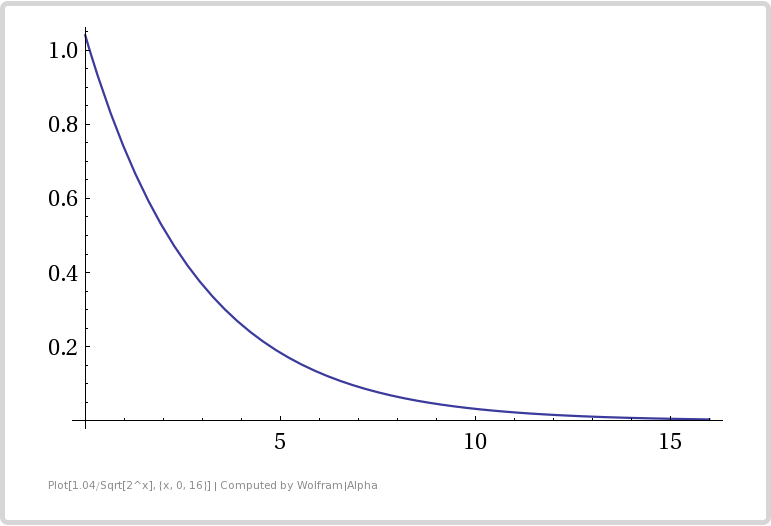
From the table and the graph you can see that adding bits (registers) gives diminishing returns in error reduction. It’s especially diminishing because whenever we add another bit, we double our storage size (double the number of registers we use).
This shows us that this algorithm is great at counting a large number of uniques, since one byte per counter can count up to about 2^256 (2^2^8) uniques, but it isn’t super great at getting a low error rate. If you are ok with about 2% accuracy, the storage space needed is pretty small though!
Remember the claim at the top of this post?
“…the new algorithm makes it possible to estimate cardinalities well beyond 10^9 with a typical accuracy of 2% while using a memory of only 1.5 kilobytes”
Looking at the bits used / error table, you can see 11 bits, or 2048 registers, gives just a little over 2% accuracy.
If you are using 32 bits of hash to look for runs of zeros, you can use 6 bit registers to store the longest run seen, if you want to waste a bit to be able to store 0-32 instead of just 0-31.
So, 2048 registers * 6 bits = 12288 bits of register storage needed. That is 1536 bytes, or exactly 1.5KB.
You could count up to ~4 billion uniques (2^32) with that configuration, but error increases as you get closer to that limit, so I think that’s why they limited their statement to counting ~1 billion uniques (10^9).
Estimating Counts
The math behind the count estimation is a bit complex (check the paper in the links section for more info!) but part of how it works is it uses the harmonic mean to average the data from the registers together. Since there is randomness involved, and differences in our run lengths means being off by exponential amounts, the harmonic mean is great at filtering out large outliers due to the random fluctuations. Fluctuation to the “too small” end won’t matter too much since it will be over-written by other values since we are storing the maximum value seen. Fluctuations to the “too large” end are mitigated with harmonic mean.
Here’s some pseudo code for estimating the count. Note that we are storing the position of the first 1 in the registers, not storing the run length of zeros. That’s an important distinction because it means the number is 1 higher than it would be otherwise, which if you get it wrong makes your estimation half as large as it should be. It also means that you know if you see a zero register, that it is uninitialized and hasn’t seen a value yet.
Alpha = 0.7213 / (1 + 1.079 / NumRegisters)
Sum = 0
for i = 0 to NumRegisters
  Sum = Sum + pow(2, -Register[i])

Estimation = Alpha * NumRegisters^2 / Sum

// do small range correction
if Estimation < 5 / 2 * NumRegisters
{
  if NumEmptyRegisters > 0
    Estimation = NumRegisters * ln(NumRegisters / NumEmptyRegisters)
}
// do large range correction
else if Estimation > 2^32 / 30
{
  Estimation = -2^32 * ln(1 - Estimation/ 2^32);
}
Small range correction is there because when not enough registers have been filled in (they haven’t gotten any data yet), the normal algorithm path has expected error greater than 1.04. Large range correction is there for the same reason, but on the high end side, when the registers are saturated.
Set Operations
You can do set operations on hyperloglog objects so long as they use the same number of registers, same sized registers, and same hashing algorithm.
There’s a link in the links section at the end of this post that shows you how to resize the number of registers so that you can do set operations on HLL objects that have different numbers of registers.
Union
Taking a union of two HLL objects is actually really simple.
If you have two HLL objects A and B, that you want to union to get C, all you do is take the maximum bucket value from A and B and store it in C. Check out this pseudocode to see what i mean:
for i = 0 to NumRegisters
  C.Register[i] = Max(A.Register[i], B.Register[i])
The neat thing about doing this union is that it is LOSSLESS and doesn’t introduce any new error. Doing a union of two HLL objects is just the same as if you had a third HLL object that processed all the same objects that A and B both processed.
Intersection
To do an intersection is a tiny bit trickier, but not by much. We have to use what is called the Inclusion-Exclusion Principle (check links section for more info).
Using that principle, we can estimate the count of how many items are in the intersection, but we can’t get a HLL object representing the intersection of the two objects unfortunately.
The formula is this:
Count(Intersection(A,B)) = Count(A) + Count(B) – Count(Union(A,B))
And here’s some more pseudocode to show you how to do it:
C = Union(A,B)
IntersectionCountEstimate = A.CountEstimate() + B.CountEstimate() - C.CountEstimate()
Pretty simple eh?
At the beginning I mentioned that KMV was actually better at intersections than HyperLogLog. The reason for that is because with KMV, you have a small, random sample range from both objects, and you can do an intersection between those two ranges and get your result.
KMV really starts to shine when you need to do an intersection between more than 2 or 3 lists, because using the inclusion-exclusion principle causes a combinatorial explosion, while the KMV intersection easily extends for N sets.
Jaccard Index
There’s no special trick to calculating the Jaccard Index, as per usual it’s just:
JaccardIndex = Count(Intersection(A,B)) / Count(Union(A,B))
Which will give you a value from 0 to 1 indicating how similar the two sets A and B are, where 1 is totally the same, and 0 is completely different. In the case of HLL, this is an estimated Jaccard Index of course, not the actual value!
Contains Percent
I was noticing in runs of the sample code below that while the union operation had pretty decent error levels, the intersection operation had not so great error levels and thus the Jaccard Index wasn’t very accurate either. This is mostly due to the fact that the intersection levels were pretty small, so if you had +1 or -1, that came out to be a large percentage of the actual value.
Despite having a reasonable explanation that diminished the actual impact of the “high error levels”, I wanted to see if I could come up with a different similarity metric and see how the error rate was on it.
What I came up with was a “Contains Percent”, which is the percentage of how many items in A are contained in B. You calculate it like this:
ContainsPercent = Count(Intersection(A,B)) / Count(A)
Since it uses the intersection value (that is not so accurate), it didn’t give great results, but I wanted to mention it because it actually is a completely different measurement than Jaccard Index with different meaning. All of the items in A could be in B, which would give it a “ContainsPercent” of 1.0, but B may have 10 times as many items that don’t appear in A, which would make the Jaccard Index very low.
In some cases, you may want to use the information that the Jaccard Index represents to make decisions, and in other cases you may want this “Contains Percent” metric, or maybe even something else.
It’s a bit subtle, but it’s good to think about what it is that you are actually looking for if using these things in actual production code (:
Estimating Set Membership
So, HLL is NOT a bloom filter, but can it still be used like one?
The answer is yes, but I don’t have a whole lot of information about the formal accuracy of that.
Basically how you’d do this is create a temporary HLL object, make it store the single item you want to check the other HLL for set membership of, and then you’d do an estimated intersection count between the two HLL objects.
As crazy as it sounds, it looks like redis exposes this functionality and says it is pretty accurate (for however many registers they used anyways), which is pretty neat:
Redis: PFCOUNT
Dot Product
The dot product between two sets (or multi sets – where you have a count associated with each item) can be really useful to help gauge the similarity between the two sets.
You can do a dot product operation between two HLL objects too. If you think about it, getting the dot product between two HLL objects is the same as getting the estimated count of the intersection between those two objects.
Example Code
Here is some example code in C++ that allows you to do HyperLogLog. It includes only standard include files so has no dependencies and is in a single file for convenience.
I use a hash called MurmurHash3 to generate 128 bits of hash, 32 bits of which are used to generate the register index, and the remaining 96 bits are used for looking at runs of zeros.
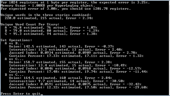
Below the code is the output of a run of this program
#include <array>
#include <string>
#include <assert.h>
#include <unordered_set>
#include <stdint.h>
#include <memory>

// microsoft only, for _BitScanForward to quickly find the index of the first 1 bit
// Use clz in gcc
#include <intrin.h>

//=====================================================================================================
// MurmurHash3
//=====================================================================================================

// from https://code.google.com/p/smhasher/source/browse/trunk/MurmurHash3.cpp
// note that this 128 bit MurmurHash3 is optimized for x86.  There is a version at the above link
// optimized for x64 as well, but it gives different output for the same input.

#define ROTL32(x,y)     _rotl(x,y)

inline uint32_t getblock32 (const uint32_t * p, int i)
{
    return p[i];
}

inline uint32_t fmix32 (uint32_t h)
{
    h ^= h >> 16;
    h *= 0x85ebca6b;
    h ^= h >> 13;
    h *= 0xc2b2ae35;
    h ^= h >> 16;

    return h;
}

void MurmurHash3_x86_128 (const void * key, const int len,
    uint32_t seed, std::array<uint32_t, 4> & out)
{
    const uint8_t * data = (const uint8_t*)key;
    const int nblocks = len / 16;

    uint32_t h1 = seed;
    uint32_t h2 = seed;
    uint32_t h3 = seed;
    uint32_t h4 = seed;

    const uint32_t c1 = 0x239b961b;
    const uint32_t c2 = 0xab0e9789;
    const uint32_t c3 = 0x38b34ae5;
    const uint32_t c4 = 0xa1e38b93;

    //----------
    // body

    const uint32_t * blocks = (const uint32_t *)(data + nblocks * 16);

    for (int i = -nblocks; i; i++)
    {
        uint32_t k1 = getblock32(blocks, i * 4 + 0);
        uint32_t k2 = getblock32(blocks, i * 4 + 1);
        uint32_t k3 = getblock32(blocks, i * 4 + 2);
        uint32_t k4 = getblock32(blocks, i * 4 + 3);

        k1 *= c1; k1 = ROTL32(k1, 15); k1 *= c2; h1 ^= k1;

        h1 = ROTL32(h1, 19); h1 += h2; h1 = h1 * 5 + 0x561ccd1b;

        k2 *= c2; k2 = ROTL32(k2, 16); k2 *= c3; h2 ^= k2;

        h2 = ROTL32(h2, 17); h2 += h3; h2 = h2 * 5 + 0x0bcaa747;

        k3 *= c3; k3 = ROTL32(k3, 17); k3 *= c4; h3 ^= k3;

        h3 = ROTL32(h3, 15); h3 += h4; h3 = h3 * 5 + 0x96cd1c35;

        k4 *= c4; k4 = ROTL32(k4, 18); k4 *= c1; h4 ^= k4;

        h4 = ROTL32(h4, 13); h4 += h1; h4 = h4 * 5 + 0x32ac3b17;
    }

    //----------
    // tail

    const uint8_t * tail = (const uint8_t*)(data + nblocks * 16);

    uint32_t k1 = 0;
    uint32_t k2 = 0;
    uint32_t k3 = 0;
    uint32_t k4 = 0;

    switch (len & 15)
    {
    case 15: k4 ^= tail[14] << 16;
    case 14: k4 ^= tail[13] << 8;
    case 13: k4 ^= tail[12] << 0;
        k4 *= c4; k4 = ROTL32(k4, 18); k4 *= c1; h4 ^= k4;

    case 12: k3 ^= tail[11] << 24;
    case 11: k3 ^= tail[10] << 16;
    case 10: k3 ^= tail[9] << 8;
    case  9: k3 ^= tail[8] << 0;
        k3 *= c3; k3 = ROTL32(k3, 17); k3 *= c4; h3 ^= k3;

    case  8: k2 ^= tail[7] << 24;
    case  7: k2 ^= tail[6] << 16;
    case  6: k2 ^= tail[5] << 8;
    case  5: k2 ^= tail[4] << 0;
        k2 *= c2; k2 = ROTL32(k2, 16); k2 *= c3; h2 ^= k2;

    case  4: k1 ^= tail[3] << 24;
    case  3: k1 ^= tail[2] << 16;
    case  2: k1 ^= tail[1] << 8;
    case  1: k1 ^= tail[0] << 0;
        k1 *= c1; k1 = ROTL32(k1, 15); k1 *= c2; h1 ^= k1;
    };

    //----------
    // finalization

    h1 ^= len; h2 ^= len; h3 ^= len; h4 ^= len;

    h1 += h2; h1 += h3; h1 += h4;
    h2 += h1; h3 += h1; h4 += h1;

    h1 = fmix32(h1);
    h2 = fmix32(h2);
    h3 = fmix32(h3);
    h4 = fmix32(h4);

    h1 += h2; h1 += h3; h1 += h4;
    h2 += h1; h3 += h1; h4 += h1;

    out[0] = h1;
    out[1] = h2;
    out[2] = h3;
    out[3] = h4;
}

struct SMurmurHash3
{
    std::array<uint32_t, 4> HashBytes (const void *key, size_t len)
    {
        // use a random 32 bit number as the seed (salt) of the hash.
        // Gotten from random.org
        // https://www.random.org/cgi-bin/randbyte?nbytes=4&format=h
        static const uint32_t c_seed = 0x2e715b3d;

        // MurmurHash3 doesn't do well with small input sizes, so if the input is too small,
        // make it longer in a way that hopefully doesn't cause likely collisions.
        // "the" hashed before the fix (notice the last 3 are the same)
        //  0x45930d0e
        //  0xfc76ee5b
        //  0xfc76ee5b
        //  0xfc76ee5b
        // and after the fix:
        //  0x70220da0
        //  0xe7d0664a
        //  0xb4e4d832
        //  0x25940640
        std::array<uint32_t, 4> ret;
        static const size_t c_minLen = 16;
        if (len < c_minLen)
        {
            unsigned char buffer[c_minLen];

            for (size_t i = 0; i < len; ++i)
                buffer[i] = ((unsigned char*)key)[i];

            for (size_t i = len; i < c_minLen; ++i)
                buffer[i] = buffer[i%len] + i;

            MurmurHash3_x86_128(buffer, c_minLen, c_seed, ret);
        }
        else
        {
            MurmurHash3_x86_128(key, len, c_seed, ret);
        }

        return ret;
    }

    template <typename T>
    std::array<uint32_t, 4> operator() (const T &object);

    template <>
    std::array<uint32_t, 4> operator() <std::string> (const std::string &object)
    {
        return HashBytes(object.c_str(), object.length());
    }

    // NOTE: if you need to hash other object types, just make your own template specialization here
};

//=====================================================================================================
// The CHyperLogLog class
//=====================================================================================================
//
// TKEY is the type of objects to keep track of
// NUMREGISTERBITS is how many bits of the hash are used to index into registers.  It also controls
//   how many registers there are since that count is 2^NUMREGISTERBITS
// HASHER controls how the keys are hashed
//
template <typename TKEY, size_t NUMREGISTERBITS, typename HASHER>
class CHyperLogLog
{
public:
    CHyperLogLog()
        : m_counts{} // init counts to zero
    { }

    // friends
    template <typename TKEY, size_t NUMREGISTERBITS, typename HASHER>
    friend float UnionCountEstimate (const CHyperLogLog<TKEY, NUMREGISTERBITS, HASHER>& A, const CHyperLogLog<TKEY, NUMREGISTERBITS, HASHER>& B);

    // constants
    static const size_t c_numRegisters = 1 << NUMREGISTERBITS;
    static const size_t c_registerMask = (c_numRegisters - 1);

    // interface
    void AddItem (const TKEY& item)
    {
        // because 2^32 does not fit in 32 bits
        static_assert(NUMREGISTERBITS < 32, "CHyperLogLog must use fewer than 32 register bits");

        // make as many hashed bits as we need
        std::array<uint32_t, 4> hash = HASHER()(item);

        // use the highest 32 bits for getting our register index
        unsigned int registerIndex = hash[3] & c_registerMask;

        // use the other 96 bits as our "unique number" corresponding to our object.  Note that we
        // don't use the high 32 bits that we've already used for the register index because that
        // would bias our results.  Certain values seen would ONLY get tracked by specific registers.
        // That's ok though that we are only using 96 bits because that is still an astronomically large
        // value.  Most HyperLogLog implementations use only 32 bits, while google uses 64 bits.  We are
        // doing even larger with 96 bits.
        // 2^(bits) = how many unique items you can track.
        //
        // 2^32  = 4 billion <--- what most people use
        // 2^64  = 18 billion billion <--- what google uses
        // 2^96  = 79 billion billion billion <--- what we are using
        // 2^128 = 340 billion billion billion billion <--- way huger than anyone needs. Beyond astronomical.

        // Figure out where the highest 1 bit is
        unsigned long bitSet = 0;
        if (_BitScanForward(&bitSet, hash[0]))
            bitSet += 1;
        else if (_BitScanForward(&bitSet, hash[1]))
            bitSet += 32 + 1;
        else if (_BitScanForward(&bitSet, hash[2]))
            bitSet += 64 + 1;

        // store the highest seen value for that register
        assert(bitSet < 256);
        unsigned char value = (unsigned char)bitSet;
        if (m_counts[registerIndex] < value)
            m_counts[registerIndex] = value;

    }

    unsigned int EmptyRegisterCount () const
    {
        unsigned int ret = 0;
        std::for_each(m_counts.begin(), m_counts.end(), [&] (unsigned char count) {
            if (count == 0)
                ret++;
        });
        return ret;
    }

    float GetCountEstimation () const
    {
        // calculate dv estimate
        const float c_alpha = 0.7213f / (1.0f + 1.079f / c_numRegisters);
        float sum = 0.0f;
        std::for_each(m_counts.begin(), m_counts.end(), [&](unsigned char count) {
            sum += std::pow(2.0f, -(float)count);
        });

        float dv_est = c_alpha * ((float)c_numRegisters / sum) * (float)c_numRegisters;

        // small range correction
        if (dv_est < 5.0f / 2.0f * (float)c_numRegisters)
        {
            // if no empty registers, use the estimate we already have
            unsigned int emptyRegisters = EmptyRegisterCount();
            if (emptyRegisters == 0)
                return dv_est;

            // balls and bins correction
            return (float)c_numRegisters * log((float)c_numRegisters / (float)emptyRegisters);
        }

        // large range correction
        if (dv_est > 143165576.533f) // 2^32 / 30
            return -pow(2.0f, 32.0f) * log(1.0f - dv_est / pow(2.0f, 32.0f));

        return dv_est;
    }

private:
    std::array<unsigned char, c_numRegisters> m_counts;
};

// there seem to be numerical problems when using 26 bits or larger worth of registers
typedef CHyperLogLog<std::string, 10, SMurmurHash3> TCounterEstimated;
typedef std::unordered_set<std::string> TCounterActual;

//=====================================================================================================
// Set Operations
//=====================================================================================================

template <typename TKEY, size_t NUMREGISTERBITS, typename HASHER>
float UnionCountEstimate (
    const CHyperLogLog<TKEY, NUMREGISTERBITS, HASHER>& A,
    const CHyperLogLog<TKEY, NUMREGISTERBITS, HASHER>& B)
{
    // dynamically allocate our hyperloglog object to not bust the stack if you are using a lot of registers.
    std::unique_ptr<CHyperLogLog<TKEY, NUMREGISTERBITS, HASHER>> temp =
        std::make_unique<CHyperLogLog<TKEY, NUMREGISTERBITS, HASHER>>();

    // To make a union between two hyperloglog objects that have the same number of registers and use
    // the same hash, just take the maximum of each register between the two objects.  This operation is
    // "lossless" in that you end up with the same registers as if you actually had another object
    // that tracked the items each individual object tracked.
    for (size_t i = 0; i < (*temp).c_numRegisters; ++i)
        (*temp).m_counts[i] = std::max(A.m_counts[i], B.m_counts[i]);
    return (*temp).GetCountEstimation();
}

template <typename TKEY, size_t NUMREGISTERBITS, typename HASHER>
float IntersectionCountEstimate (
    const CHyperLogLog<TKEY, NUMREGISTERBITS, HASHER>& A,
    const CHyperLogLog<TKEY, NUMREGISTERBITS, HASHER>& B)
{
    // We have to use the inclusion-exclusion principle to get an intersection estimate
    // count(Intersection(A,B)) = (count(A) + count(B)) - count(Union(A,B))
    // http://en.wikipedia.org/wiki/Inclusion%E2%80%93exclusion_principle

    return (A.GetCountEstimation() + B.GetCountEstimation()) - UnionCountEstimate(A, B);
}

float UnionCountActual (const TCounterActual& A, const TCounterActual& B)
{
    TCounterActual temp;
    std::for_each(A.begin(), A.end(), [&] (const TCounterActual::key_type &s){temp.insert(s);});
    std::for_each(B.begin(), B.end(), [&] (const TCounterActual::key_type &s){temp.insert(s);});
    return (float)temp.size();
}

float IntersectionCountActual (const TCounterActual& A, const TCounterActual& B)
{
    float ret = 0;
    std::for_each(A.begin(), A.end(), [&](const TCounterActual::key_type &s)
    {
        if (B.find(s) != B.end())
            ++ret;
    });
    return ret;
}

//=====================================================================================================
// Error Calculations
//=====================================================================================================

float ExpectedError (size_t numRegisters)
{
    return 1.04f / ((float)(sqrt((float)numRegisters)));
}

float IdealRegisterCount (float expectedError)
{
    return 676.0f / (625.0f * expectedError * expectedError);
}

//=====================================================================================================
// Driver Program
//=====================================================================================================

template <typename L>
void ForEachWord(const std::string &source, L& lambda)
{
    size_t prev = 0;
    size_t next = 0;

    while ((next = source.find_first_of(" ,.-":n", prev)) != std::string::npos)
    {
        if ((next - prev != 0))
        {
            std::string word = source.substr(prev, next - prev);
            std::transform(word.begin(), word.end(), word.begin(), ::tolower);
            lambda(word);
        }
        prev = next + 1;
    }

    if (prev < source.size())
    {
        std::string word = source.substr(prev);
        std::transform(word.begin(), word.end(), word.begin(), ::tolower);
        lambda(word);
    }
}

template <typename T>
const char *CalculateError (const T&estimate, const T&actual)
{
    float error = 100.0f * ((float)estimate - (float)actual) / (float)actual;
    if (std::isnan(error) || std::isinf(error))
        return "undef";

    // bad practice to return a static local string, dont do this in production code!
    static char ret[256];
    sprintf_s(ret, sizeof(ret), "%0.2f%%", error);
    return ret;
}

char *BytesToHumanReadable (size_t bytes)
{
    // bad practice to return a static local string, dont do this in production code!
    static char ret[256];
    if (bytes >= 1024 * 1024 * 1024)
        sprintf_s(ret, sizeof(ret), "%0.2fGB", ((float)bytes) / (1024.0f*1024.0f*1024.0f));
    else if (bytes >= 1024 * 1024)
        sprintf_s(ret, sizeof(ret), "%0.2fMB", ((float)bytes) / (1024.0f*1024.0f));
    else if (bytes >= 1024)
        sprintf_s(ret, sizeof(ret), "%0.2fKB", ((float)bytes) / (1024.0f));
    else
        sprintf_s(ret, sizeof(ret), "%u Bytes", bytes);
    return ret;
}

void WaitForEnter()
{
    printf("nPress Enter to quit");
    fflush(stdin);
    getchar();
}

// These one paragraph stories are from http://birdisabsurd.blogspot.com/p/one-paragraph-stories.html

// The Dino Doc : http://birdisabsurd.blogspot.com/2011/11/dino-doc.html (97 words)
const char *g_storyA =
"The Dino Doc:n"
"Everything had gone according to plan, up 'til this moment. His design team "
"had done their job flawlessly, and the machine, still thrumming behind him, "
"a thing of another age, was settled on a bed of prehistoric moss. They'd "
"done it. But now, beyond the protection of the pod and facing an enormous "
"tyrannosaurus rex with dripping jaws, Professor Cho reflected that, had he "
"known of the dinosaur's presence, he wouldn't have left the Chronoculator - "
"and he certainly wouldn't have chosen "Stayin' Alive", by The Beegees, as "
"his dying soundtrack. Curse his MP3 player";

// The Robot: http://birdisabsurd.blogspot.com/2011/12/robot.html (121 words)
const char *g_storyB =
"The Robot:n"
"The engineer watched his robot working, admiring its sense of purpose.It knew "
"what it was, and what it had to do.It was designed to lift crates at one end "
"of the warehouse and take them to the opposite end.It would always do this, "
"never once complaining about its place in the world.It would never have to "
"agonize over its identity, never spend empty nights wondering if it had been "
"justified dropping a promising and soul - fulfilling music career just to "
"collect a bigger paycheck.And, watching his robot, the engineer decided that "
"the next big revolution in the robotics industry would be programming "
"automatons with a capacity for self - doubt.The engineer needed some company.";

// The Internet: http://birdisabsurd.blogspot.com/2011/11/internet.html (127 words)
const char *g_storyC =
"The Internet:n"
"One day, Sandra Krewsky lost her mind.Nobody now knows why, but it happened - "
"and when it did, Sandra decided to look at every page on the Internet, "
"insisting that she wouldn't eat, drink, sleep or even use the washroom until "
"the job was done. Traps set in her house stalled worried family members, and by "
"the time they trounced the alligator guarding her bedroom door - it managed to "
"snap her neighbour's finger clean off before going down - Sandra was already "
"lost… though the look of despair carved in her waxen features, and the cat "
"video running repeat on her flickering computer screen, told them everything "
"they needed to know.She'd seen too much. She'd learned that the Internet "
"played for keeps.";

int main (int argc, char **argv)
{
    // show basic info regarding memory usage, precision, etc
    printf("For %u registers at 1 byte per register, the expected error is %0.2f%%.n",
        TCounterEstimated::c_numRegisters,
        100.0f * ExpectedError(TCounterEstimated::c_numRegisters)
    );
    printf("Memory Usage = %s per HyperLogLog object.n", BytesToHumanReadable(TCounterEstimated::c_numRegisters));
    static const float c_expectedError = 0.03f;
    printf("For expected error of %0.2f%%, you should use %0.2f registers.nn",
        100.0f*c_expectedError,
        IdealRegisterCount(c_expectedError)
    );

    // populate our data structures
    // dynamically allocate estimate so we don't bust the stack if we have a large number of registers
    std::unique_ptr<TCounterEstimated> estimateTotal = std::make_unique<TCounterEstimated>();
    std::unique_ptr<TCounterEstimated> estimateA = std::make_unique<TCounterEstimated>();
    std::unique_ptr<TCounterEstimated> estimateB = std::make_unique<TCounterEstimated>();
    std::unique_ptr<TCounterEstimated> estimateC = std::make_unique<TCounterEstimated>();
    TCounterActual actualTotal;
    TCounterActual actualA;
    TCounterActual actualB;
    TCounterActual actualC;
    {
        auto f = [&](const std::string &word)
        {
            estimateTotal->AddItem(word);
            actualTotal.insert(word);
        };

        auto fA = [&](const std::string &word)
        {
            estimateA->AddItem(word);
            actualA.insert(word);
            f(word);
        };

        auto fB = [&](const std::string &word)
        {
            estimateB->AddItem(word);
            actualB.insert(word);
            f(word);
        };

        auto fC = [&](const std::string &word)
        {
            estimateC->AddItem(word);
            actualC.insert(word);
            f(word);
        };

        ForEachWord(g_storyA, fA);
        ForEachWord(g_storyB, fB);
        ForEachWord(g_storyC, fC);
    }

    // Show unique word counts for the three combined stories
    {
        float estimateCount = estimateTotal->GetCountEstimation();
        float actualCount = (float)actualTotal.size();
        printf("Unique words in the three stories combined:n");
        printf("  %0.1f estimated, %.0f actual, Error = %snn",
            estimateCount,
            actualCount,
            CalculateError(estimateCount, actualCount)
        );
    }

    // show unique word counts per story
    {
        printf("Unique Word Count Per Story:n");
        auto g = [](const char *name, const TCounterEstimated &estimate, const TCounterActual &actual)
        {
            float estimateCount = estimate.GetCountEstimation();
            float actualCount = (float)actual.size();
            printf("  %s = %0.1f estimated, %.0f actual, Error = %sn",
                name,
                estimateCount,
                actualCount,
                CalculateError(estimateCount, actualCount)
            );
        };

        g("A", *estimateA, actualA);
        g("B", *estimateB, actualB);
        g("C", *estimateC, actualC);
    }

    // Set Operations
    {
        printf("nSet Operations:n");

        auto f = [] (
            const char *name1,
            const TCounterEstimated &estimate1,
            const TCounterActual &actual1,
            const char *name2,
            const TCounterEstimated &estimate2,
            const TCounterActual &actual2
        )
        {
            printf("  %s vs %s...n", name1, name2);

            // union
            float estimateUnionCount = UnionCountEstimate(estimate1, estimate2);
            float actualUnionCount = UnionCountActual(actual1, actual2);
            printf("    Union: %0.1f estimated, %.0f actual, Error = %sn",
                estimateUnionCount,
                actualUnionCount,
                CalculateError(estimateUnionCount, actualUnionCount)
            );

            // intersection
            float estimateIntersectionCount = IntersectionCountEstimate(estimate1, estimate2);
            float actualIntersectionCount = IntersectionCountActual(actual1, actual2);
            printf("    Intersection: %0.1f estimated, %.0f actual, Error = %sn",
                estimateIntersectionCount,
                actualIntersectionCount,
                CalculateError(estimateIntersectionCount, actualIntersectionCount)
            );

            // jaccard index
            float estimateJaccard = estimateIntersectionCount / estimateUnionCount;
            float actualJaccard = actualIntersectionCount / actualUnionCount;
            printf("    Jaccard Index: %0.4f estimated, %.4f actual, Error = %sn",
                estimateJaccard,
                actualJaccard,
                CalculateError(estimateJaccard, actualJaccard)
            );

            // Contains Percent.
            // What percentage of items in A are also in B?
            float estimateSim = estimateIntersectionCount / estimate1.GetCountEstimation();
            float actualSim = actualIntersectionCount / actual1.size();
            printf("    Contains Percent: %0.2f%% estimated, %0.2f%% actual, Error = %sn",
                100.0f*estimateSim,
                100.0f*actualSim,
                CalculateError(estimateSim, actualSim)
            );
        };

        f("A", *estimateA, actualA, "B", *estimateB, actualB);
        f("A", *estimateA, actualA, "C", *estimateC, actualC);
        f("B", *estimateB, actualB, "C", *estimateC, actualC);
    }

    WaitForEnter();
    return 0;
}
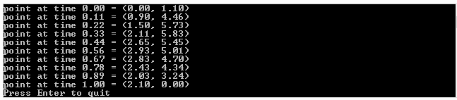
Here is the output of the above program:
Want More?
As per usual, the rabbit hole goes far deeper than what I’ve shown. Check out the links below to go deeper!
HyperLogLog Research Paper
Combining HLL and KMV to Get The Best of Both
Doubling the Count of HLL Registers on the Fly
Set Operations on HLLs of Different Sizes
Interactive HyperLogLog Demo
Interactive HyperLogLog Union Demo
HyperLogLog++ Research Paper
HyperLogLog++ Analyzed
Wikipedia: Inclusion Exclusion Principle
Coin Flipping
Wikipedia: MurmurHash3
MurmurHash3 C++ Source Code


 and
and  at time
  , where
  .
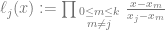
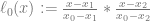
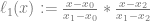
. . A quadratic curve is just a linear interpolation between two curves of degree 1 (aka linear curves). Specifically, you take a linear interpolation between
  , and a linear interpolation between
  , and then take a linear interpolation between those two results. That will give you your quadratic curve.
 . A cubic curve is just a linear interpolation between two quadratic curves. Specifically, the first quadratic curve is defined by control points
  .
.
 . A quartic curve is just a linear interpolation between two cubic curves. The first cubic curve is defined by control points
  .
.

 is just
  )
)

 and
and  , using the alpha of the pixel you are writing to determine the weighting for the lerp.
 is already multipled by
  which results in slightly less math:


 are the weightings associated with those control points.
 .
. or
or  or
or  .
. , instead of
  , we come up with the equation in the next section.
 for ANY value


 case. The next row down is “1,2,1” which is the constants multiplied by each term for the
  case. Lastly the next row down (fourth row) is “1,3,3,1” which is the constants multiplied by each term for the
  case. Essentially, you just use the
  th tow of pascals triangle to come up with the constants to multiply each term by.
 , and then multiply each term by a unique control point (A,B,C,etc). After you have your equation, you can optionally replace all


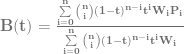
 (Sigma, going from 0 to n) means that you are going to sum (add) together n+1 terms (it includes both 0 and n), using i as the loop variable in your summation. It’s basically a for loop, adding together each iteration of the for loop. Everything that comes after is what happens during each iteration of the for loop that gets summed together.
 part means to take the ith number from the (n+1)th row of Pascal’s triangle. More formally, this specifies to use specific binomial coefficients.
 means that you multiply the binomial coefficient by s to the (n-i)th power, and t to the ith power. This is the same as saying s starts at power n and counts down left to right, while t starts at 0 and counts up left to right. This fits the pattern we saw above in binomial expansion.
 which means to use the ith P. So, P is basically an array with n+1 elements. This array is the control points, so each P is a different control point.