Generating Blue Noise Sample Points With Mitchell’s Best Candidate Algorithm

Lately I’ve been eyeball deep in noise, ordered dithering and related topics, and have been learning some really interesting things.

As the information coalesces it’ll become apparent whether there is going to be a huge mega post coming, or if there will be several smaller ones.

In the meantime, I wanted to share this bite sized chunk of information.

Three sampling patterns that are most often used when sampling (say, when numerically integrating a lighting function for graphics/rendering purposes) are: regular samples, white noise samples, and blue noise samples.

Regular Sampling

Regular sampling just means evenly spacing the samples. This sampling strategy can suffer from aliasing, but gives good coverage of the sample space.

Here are 256, 1024 and 4096 samples:


Here are those samples taken from a source image:


Here is the DFT (frequency amplitude) of those samples:


White Noise Sampling

White noise sampling just chooses random numbers for where to place the samples.
The random numbers are uniformly distributed, meaning they are just plain vanilla random numbers where each number is equally likely to come up.

White noise sampling can make for noisy results, and suffers from the fact that white noise sample points can clump together and leave empty space. Clumped sample points give redundant information while empty space is information that you are lacking in the sample space. In general, noise is often desired over aliasing though, so white noise samples are generally preferred over regular sampling. Monte Carlo integration also requires random samples.

White noise is called white noise because it contains all frequencies approximately evenly, like how white light is made up of all frequencies of light.

Here are 256, 1024 and 4096 samples:


Here are those samples taken from a source image:


Here is the DFT (frequency amplitude) of those samples:


Blue Noise Sampling

Lastly is blue noise sampling which is somewhere between regular sampling and white noise sampling. Blue noise sampling has randomly placed points like white noise does, but the randomly placed points are approximately evenly spaced, which is more like regular sampling.

Things like low discrepancy sequences, stratified sampling, and jittered regular sampling mimic blue noise, and are often a cheaper alternative when an approximation is acceptable. More info on low discrepancy sequences is available on my post here: When Random Numbers Are Too Random: Low Discrepancy Sequences

Blue noise is called blue noise because it contains higher amounts of higher frequencies and lower amounts of lower frequencies. This is the same of blue light, which contains higher frequency (bluer) light.

Here are 256, 1024 and 4096 samples:


Here are those samples taken from a source image:


Here is the DFT (frequency amplitude) of those samples:


Comparison

Imagine you were a robot with 4096 light/color sensors. Which of the arrangements below do you think would give you the best information about the world around you with that number of sensors?


To me, the regular grid and the blue noise are a bit of a coin toss, while the white noise version is awful.

The regular grid does seem to show me straight lined things better (the road, sidewalk, etc), but it makes non straight lined things – like the trees – look blocky. The blue noise grid does the reverse and makes straight things look wavy, while making it easier to see the true shape of non straight things.

Mathematically, blue noise is superior sampling, so maybe this example isn’t the best way to show the value of blue noise.

Here is the real image:

Apparently the photo-receptors in our eyes are arranged in a blue noise pattern. Some people say this is why blue noise is more agreeable with our perception, but since it also helps numerical integration converge faster for lower sample counts (compared to white noise – which wins out with larger sample counts BTW!), it seems like there is a more fundamental reason which would cause an evolutionary advantage for them to be arranged that way in the first place.

Generating Blue Noise Sample Points

The obvious question is: I know how to make uniform and random sample points. How do I make blue noise sample points?

There are multiple ways to do it, but a method that I find very easy to understand and to implement is “Mitchell’s Best Candidate Algorithm”.

The algorithm is as follows:

  1. Place a random sample point as the first sample point.
  2. Generate some number of random dots as candidates to be the next sample point.
  3. Whichever of these dots is farthest away from the closest existing sample point is the winner. Place that dot as the new sample point.
  4. GOTO 2 and Repeat until you have as many sample points as you want.

The algorithm is pretty simple, but there are two other important details that are needed to give you good results:

  • When calculating distance between dots, you need to consider wrap around. More info on how to do that here: Calculating the Distance Between Points in “Wrap Around” (Toroidal) Space.
  • The number of candidates you generate should scale up with the number of existing sample points. As the original paper describing this technique says, doing that helps ensure that the statistics of your sample points stay constant as the number of sample points changes.

When I first tried to get this algorithm working, I was generating a fixed number of candidates each time. That gave me these pretty terrible results:

However, when I multiplied the number of existing sample points by a constant “m” as the number of sample points to generate, I got much better results, even when m was 1! (Note: m=0 is the same as white noise in this image. I did NumSamples*m+1 candidates each time.)

Related Computer Graphics Stack Exchange Question: Mitchell’s Best Candidate Algorithm

If you store existing sample points in a grid, you can speed up the algorithm since it will be faster to find the closest point to a candidate. In the implementation on this post I didn’t do that.

You may be able to multithread this algorithm but I haven’t tried it. The idea would be if you needed to make and test N candidates, that you could split that among M threads, so long as N was large enough to make that worth while. I didn’t do that in this post.

Lastly, instead of working with distance, you can work with SQUARED distance to avoid many unnecessary square root calculations. The example code here does that optimization.

Links

The 1991 paper that described this technique:
Spectrally optimal sampling for distribution ray tracing

Another interesting link on this algorithm:
Mitchell’s Best-Candidate

This algorithm isn’t that great for making dense sample points, or for use in dithering / stippling. Look for a future blog post about those usage cases, but for now, this is a great resource:
Free Blue Noise Textures (and info / examples on blue noise texture usage)

A physics based approach to blue noise distributed samples:
Electrostatic Half Toning

A neat read on the “void and cluster” method for generating blue noise, and also a good read on what ordered dithering is all about:
The void and cluster method for dither array generation

Source Code

Here is some simple standalone C++ source code which can generate blue noise sample points, and also generated the images used in this post.

It’s also on github (along with the source image) at https://github.com/Atrix256/RandomCode/tree/master/Mitchell

#define _CRT_SECURE_NO_WARNINGS

#include <windows.h>  // for bitmap headers.  Sorry non windows people!
#include <stdint.h>
#include <vector>
#include <complex>
#include <thread>
#include <atomic>
#include <random>
#include <array>

typedef uint8_t uint8;
typedef int64_t int64;

const float c_pi = 3.14159265359f;

//======================================================================================
struct SImageData
{
    SImageData ()
        : m_width(0)
        , m_height(0)
    { }
   
    size_t m_width;
    size_t m_height;
    size_t m_pitch;
    std::vector<uint8> m_pixels;
};

SImageData s_stippleImage;
 
//======================================================================================
struct SColor
{
    SColor (uint8 _R = 0, uint8 _G = 0, uint8 _B = 0)
        : R(_R), G(_G), B(_B)
    { }

    inline void Set (uint8 _R, uint8 _G, uint8 _B)
    {
        R = _R;
        G = _G;
        B = _B;
    }
 
    uint8 B, G, R;
};

//======================================================================================
struct SImageDataComplex
{
    SImageDataComplex ()
        : m_width(0)
        , m_height(0)
    { }
 
    size_t m_width;
    size_t m_height;
    std::vector<std::complex<float>> m_pixels;
};

//======================================================================================
std::complex<float> DFTPixel (const SImageData &srcImage, size_t K, size_t L)
{
    std::complex<float> ret(0.0f, 0.0f);
 
    for (size_t x = 0; x < srcImage.m_width; ++x)
    {
        for (size_t y = 0; y < srcImage.m_height; ++y)
        {
            // Get the pixel value (assuming greyscale) and convert it to [0,1] space
            const uint8 *src = &srcImage.m_pixels[(y * srcImage.m_pitch) + x * 3];
            float grey = float(src[0]) / 255.0f;
 
            // Add to the sum of the return value
            float v = float(K * x) / float(srcImage.m_width);
            v += float(L * y) / float(srcImage.m_height);
            ret += std::complex<float>(grey, 0.0f) * std::polar<float>(1.0f, -2.0f * c_pi * v);
        }
    }
 
    return ret;
}
 
//======================================================================================
void DFTImage (const SImageData &srcImage, SImageDataComplex &destImage)
{
    // NOTE: this function assumes srcImage is greyscale, so works on only the red component of srcImage.
    // ImageToGrey() will convert an image to greyscale.

    // size the output dft data
    destImage.m_width = srcImage.m_width;
    destImage.m_height = srcImage.m_height;
    destImage.m_pixels.resize(destImage.m_width*destImage.m_height);

    size_t numThreads = std::thread::hardware_concurrency();
    //if (numThreads > 0)
        //numThreads = numThreads - 1;

    std::vector<std::thread> threads;
    threads.resize(numThreads);

    printf("Doing DFT with %zu threads...\n", numThreads);

    // calculate 2d dft (brute force, not using fast fourier transform) multithreadedly
    std::atomic<size_t> nextRow(0);
    for (std::thread& t : threads)
    {
        t = std::thread(
            [&] ()
            {
                size_t row = nextRow.fetch_add(1);
                bool reportProgress = (row == 0);
                int lastPercent = -1;

                while (row < srcImage.m_height)
                {
                    // calculate the DFT for every pixel / frequency in this row
                    for (size_t x = 0; x < srcImage.m_width; ++x)
                    {
                        destImage.m_pixels[row * destImage.m_width + x] = DFTPixel(srcImage, x, row);
                    }

                    // report progress if we should
                    if (reportProgress)
                    {
                        int percent = int(100.0f * float(row) / float(srcImage.m_height));
                        if (lastPercent != percent)
                        {
                            lastPercent = percent;
                            printf("            \rDFT: %i%%", lastPercent);
                        }
                    }

                    // go to the next row
                    row = nextRow.fetch_add(1);
                }
            }
        );
    }

    for (std::thread& t : threads)
        t.join();

    printf("\n");
}

//======================================================================================
void GetMagnitudeData (const SImageDataComplex& srcImage, SImageData& destImage)
{
    // size the output image
    destImage.m_width = srcImage.m_width;
    destImage.m_height = srcImage.m_height;
    destImage.m_pitch = 4 * ((srcImage.m_width * 24 + 31) / 32);
    destImage.m_pixels.resize(destImage.m_pitch*destImage.m_height);
 
    // get floating point magnitude data
    std::vector<float> magArray;
    magArray.resize(srcImage.m_width*srcImage.m_height);
    float maxmag = 0.0f;
    for (size_t x = 0; x < srcImage.m_width; ++x)
    {
        for (size_t y = 0; y < srcImage.m_height; ++y)
        {
            // Offset the information by half width & height in the positive direction.
            // This makes frequency 0 (DC) be at the image origin, like most diagrams show it.
            int k = (x + (int)srcImage.m_width / 2) % (int)srcImage.m_width;
            int l = (y + (int)srcImage.m_height / 2) % (int)srcImage.m_height;
            const std::complex<float> &src = srcImage.m_pixels[l*srcImage.m_width + k];
 
            float mag = std::abs(src);
            if (mag > maxmag)
                maxmag = mag;
 
            magArray[y*srcImage.m_width + x] = mag;
        }
    }
    if (maxmag == 0.0f)
        maxmag = 1.0f;
 
    const float c = 255.0f / log(1.0f+maxmag);
 
    // normalize the magnitude data and send it back in [0, 255]
    for (size_t x = 0; x < srcImage.m_width; ++x)
    {
        for (size_t y = 0; y < srcImage.m_height; ++y)
        {
            float src = c * log(1.0f + magArray[y*srcImage.m_width + x]);
 
            uint8 magu8 = uint8(src);
 
            uint8* dest = &destImage.m_pixels[y*destImage.m_pitch + x * 3];
            dest[0] = magu8;
            dest[1] = magu8;
            dest[2] = magu8;
        }
    }
}
 
//======================================================================================
void GetPhaseData (const SImageDataComplex& srcImage, SImageData& destImage)
{
    // size the output image
    destImage.m_width = srcImage.m_width;
    destImage.m_height = srcImage.m_height;
    destImage.m_pitch = 4 * ((srcImage.m_width * 24 + 31) / 32);
    destImage.m_pixels.resize(destImage.m_pitch*destImage.m_height);
 
    // get floating point phase data, and encode it in [0,255]
    for (size_t x = 0; x < srcImage.m_width; ++x)
    {
        for (size_t y = 0; y < srcImage.m_height; ++y)
        {
            // Offset the information by half width & height in the positive direction.
            // This makes frequency 0 (DC) be at the image origin, like most diagrams show it.
            int k = (x + (int)srcImage.m_width / 2) % (int)srcImage.m_width;
            int l = (y + (int)srcImage.m_height / 2) % (int)srcImage.m_height;
            const std::complex<float> &src = srcImage.m_pixels[l*srcImage.m_width + k];
 
            // get phase, and change it from [-pi,+pi] to [0,255]
            float phase = (0.5f + 0.5f * std::atan2(src.real(), src.imag()) / c_pi);
            if (phase < 0.0f)
                phase = 0.0f;
            if (phase > 1.0f)
                phase = 1.0;
            uint8 phase255 = uint8(phase * 255);
 
            // write the phase as grey scale color
            uint8* dest = &destImage.m_pixels[y*destImage.m_pitch + x * 3];
            dest[0] = phase255;
            dest[1] = phase255;
            dest[2] = phase255;
        }
    }
}

//======================================================================================
bool ImageSave (const SImageData &image, const char *fileName)
{
    // open the file if we can
    FILE *file;
    file = fopen(fileName, "wb");
    if (!file) {
        printf("Could not save %s\n", fileName);
        return false;
    }
   
    // make the header info
    BITMAPFILEHEADER header;
    BITMAPINFOHEADER infoHeader;
   
    header.bfType = 0x4D42;
    header.bfReserved1 = 0;
    header.bfReserved2 = 0;
    header.bfOffBits = 54;
   
    infoHeader.biSize = 40;
    infoHeader.biWidth = (LONG)image.m_width;
    infoHeader.biHeight = (LONG)image.m_height;
    infoHeader.biPlanes = 1;
    infoHeader.biBitCount = 24;
    infoHeader.biCompression = 0;
    infoHeader.biSizeImage = (DWORD) image.m_pixels.size();
    infoHeader.biXPelsPerMeter = 0;
    infoHeader.biYPelsPerMeter = 0;
    infoHeader.biClrUsed = 0;
    infoHeader.biClrImportant = 0;
   
    header.bfSize = infoHeader.biSizeImage + header.bfOffBits;
   
    // write the data and close the file
    fwrite(&header, sizeof(header), 1, file);
    fwrite(&infoHeader, sizeof(infoHeader), 1, file);
    fwrite(&image.m_pixels[0], infoHeader.biSizeImage, 1, file);
    fclose(file);
  
    return true;
}

//======================================================================================
bool ImageLoad (const char *fileName, SImageData& imageData)
{
    // open the file if we can
    FILE *file;
    file = fopen(fileName, "rb");
    if (!file)
        return false;
 
    // read the headers if we can
    BITMAPFILEHEADER header;
    BITMAPINFOHEADER infoHeader;
    if (fread(&header, sizeof(header), 1, file) != 1 ||
        fread(&infoHeader, sizeof(infoHeader), 1, file) != 1 ||
        header.bfType != 0x4D42 || infoHeader.biBitCount != 24)
    {
        fclose(file);
        return false;
    }
 
    // read in our pixel data if we can. Note that it's in BGR order, and width is padded to the next power of 4
    imageData.m_pixels.resize(infoHeader.biSizeImage);
    fseek(file, header.bfOffBits, SEEK_SET);
    if (fread(&imageData.m_pixels[0], imageData.m_pixels.size(), 1, file) != 1)
    {
        fclose(file);
        return false;
    }
 
    imageData.m_width = infoHeader.biWidth;
    imageData.m_height = infoHeader.biHeight;
    imageData.m_pitch = 4 * ((imageData.m_width * 24 + 31) / 32);
 
    fclose(file);
    return true;
}

//======================================================================================
void ImageInit (SImageData& image, size_t width, size_t height)
{
    image.m_width = width;
    image.m_height = height;
    image.m_pitch = 4 * ((width * 24 + 31) / 32);
    image.m_pixels.resize(image.m_pitch * image.m_width);
    std::fill(image.m_pixels.begin(), image.m_pixels.end(), 0);
}

//======================================================================================
void SampleTest (const SImageData& image, const SImageData& samples, const char* fileName)
{
    SImageData outImage;
    ImageInit(outImage, image.m_width, image.m_height);

    for (size_t y = 0; y < image.m_height; ++y)
    {
        size_t sampleY = y % samples.m_height;
        for (size_t x = 0; x < image.m_width; ++x)
        {
            size_t sampleX = x % samples.m_width;

            const SColor* samplePixel = (SColor*)&samples.m_pixels[sampleY*samples.m_pitch + sampleX * 3];
            const SColor* imagePixel = (SColor*)&image.m_pixels[y*image.m_pitch + x * 3];

            SColor* outPixel = (SColor*)&outImage.m_pixels[y*outImage.m_pitch + x * 3];

            if (samplePixel->R == 255)
                *outPixel = *imagePixel;
        }
    }

    ImageSave(outImage, fileName);
}

//======================================================================================
inline float Distance (size_t x1, size_t y1, size_t x2, size_t y2, int imageWidth)
{
    // this returns the toroidal distance between the points
    // aka the interval [0, width) wraps around
    float dx = std::abs(float(x2) - float(x1));
    float dy = std::abs(float(y2) - float(y1));

    if (dx > float(imageWidth / 2))
        dx = float(imageWidth) - dx;

    if (dy > float(imageWidth / 2))
        dy = float(imageWidth) - dy;

    // returning squared distance cause why not
    return dx*dx + dy*dy;
}

//======================================================================================
int main (int argc, char** argv)
{
    const size_t c_imageSize = 256;
    const bool c_doDFT = true;

    const size_t c_blueNoiseSampleMultiplier = 1;

    const size_t samples1 = 256;   // 16x16
    const size_t samples2 = 1024;  // 32x32
    const size_t samples3 = 4096; // 128x128

    // load the source image
    SImageData image;
    ImageLoad("Image.bmp", image);

    // init random number generator
    std::random_device rd;
    std::mt19937 rng(rd());
    std::uniform_int_distribution<int> dist(0, c_imageSize - 1);

    // white noise
    {
        SImageData samples;
        ImageInit(samples, c_imageSize, c_imageSize);

        for (size_t i = 1; i <= samples3; ++i)
        {
            size_t x = dist(rng);
            size_t y = dist(rng);

            SColor* pixel = (SColor*)&samples.m_pixels[y*samples.m_pitch + x * 3];
            pixel->R = pixel->G = pixel->B = 255;

            if (i == samples1 || i == samples2 || i == samples3)
            {
                printf("White Noise %zu samples\n", i);

                char fileName[256];
                sprintf(fileName, "WhiteNoise_%zu.bmp", i);
                ImageSave(samples, fileName);

                sprintf(fileName, "WhiteNoise_%zu_samples.bmp", i);
                SampleTest(image, samples, fileName);

                if (c_doDFT)
                {
                    SImageDataComplex frequencyData;
                    DFTImage(samples, frequencyData);

                    SImageData magnitudeData;
                    GetMagnitudeData(frequencyData, magnitudeData);

                    sprintf(fileName, "WhiteNoise_%zu_mag.bmp", i);
                    ImageSave(magnitudeData, fileName);
                }
            }
        }
    }

    // regular samples
    {

        auto GridTest = [&] (size_t sampleCount) {
            SImageData samples;
            ImageInit(samples, c_imageSize, c_imageSize);

            size_t side = size_t(std::sqrt(float(sampleCount)));

            size_t pixels = c_imageSize / side;

            for (size_t y = 0; y < side; ++y)
            {
                size_t pixelY = y * pixels;
                for (size_t x = 0; x < side; ++x)
                {
                    size_t pixelX = x * pixels;

                    SColor* pixel = (SColor*)&samples.m_pixels[pixelY*samples.m_pitch + pixelX * 3];
                    pixel->R = pixel->G = pixel->B = 255;
                }
            }

            printf("Regular %zu samples\n", sampleCount);

            char fileName[256];
            sprintf(fileName, "Regular_%zu.bmp", sampleCount);
            ImageSave(samples, fileName);

            sprintf(fileName, "Regular_%zu_samples.bmp", sampleCount);
            SampleTest(image, samples, fileName);

            if (c_doDFT)
            {
                SImageDataComplex frequencyData;
                DFTImage(samples, frequencyData);

                SImageData magnitudeData;
                GetMagnitudeData(frequencyData, magnitudeData);

                sprintf(fileName, "Regular_%zu_mag.bmp", sampleCount);
                ImageSave(magnitudeData, fileName);
            }
        };

        GridTest(samples1);
        GridTest(samples2);
        GridTest(samples3);
    }

    // blue noise
    {
        SImageData samples;
        ImageInit(samples, c_imageSize, c_imageSize);

        std::vector<std::array<size_t, 2>> samplesPos;

        size_t percent = (size_t)-1;

        for (size_t i = 1; i <= samples3; ++i)
        {
            size_t newPercent;
            if (i <= samples1)
                newPercent = size_t(100.0f * float(i) / float(samples1));
            else if (i <= samples2)
                newPercent = size_t(100.0f * float(i - samples1) / float(samples2 - samples1));
            else
                newPercent = size_t(100.0f * float(i - samples2) / float(samples3 - samples2));
            if (percent != newPercent)
            {
                percent = newPercent;
                printf("\rGenerating Blue Noise Samples: %zu%%", percent);
            }

            // keep the candidate that is farthest from it's closest point
            size_t numCandidates = samplesPos.size() * c_blueNoiseSampleMultiplier + 1;
            float bestDistance = 0.0f;
            size_t bestCandidateX = 0;
            size_t bestCandidateY = 0;
            for (size_t candidate = 0; candidate < numCandidates; ++candidate)
            {
                size_t x = dist(rng);
                size_t y = dist(rng);

                // calculate the closest distance from this point to an existing sample
                float minDist = FLT_MAX;
                for (const std::array<size_t, 2>& samplePos : samplesPos)
                {
                    float dist = Distance(x, y, samplePos[0], samplePos[1], c_imageSize);
                    if (dist < minDist)
                        minDist = dist;
                }

                if (minDist > bestDistance)
                {
                    bestDistance = minDist;
                    bestCandidateX = x;
                    bestCandidateY = y;
                }
            }
            samplesPos.push_back({ bestCandidateX, bestCandidateY });

            SColor* pixel = (SColor*)&samples.m_pixels[bestCandidateY*samples.m_pitch + bestCandidateX * 3];
            pixel->R = pixel->G = pixel->B = 255;

            if (i == samples1 || i == samples2 || i == samples3)
            {
                printf("\nBlue Noise %zu samples\n", i);

                char fileName[256];
                sprintf(fileName, "BlueNoise_%zu.bmp", i);
                ImageSave(samples, fileName);

                sprintf(fileName, "BlueNoise_%zu_samples.bmp", i);
                SampleTest(image, samples, fileName);

                if (c_doDFT)
                {
                    SImageDataComplex frequencyData;
                    DFTImage(samples, frequencyData);

                    SImageData magnitudeData;
                    GetMagnitudeData(frequencyData, magnitudeData);

                    sprintf(fileName, "BlueNoise_%zu_mag.bmp", i);
                    ImageSave(magnitudeData, fileName);
                }
            }
        }
    }

    return 0;
}
Calculating the Distance Between Points in “Wrap Around” (Toroidal) Space

Let’s say you are trying to find the distance between two points in 2D, but that these points are in a universe that “wraps around” like old video games – leaving the screen on the right, left, top or bottom side makes you re-appear on the opposite edge.

This universe is actually shaped like a toroid, also known as a doughnut. It’s actually an impossible object, a “flat torus”, so not exactly a doughnut, but whatever.

If you imagine yourself on the surface of a doughnut, it would behave exactly this way. If you go “down” you end up where you previously considered “up”. If you go far enough “left” you end up where you previously considered “right”.

How would you calculate the distance between two points in a universe like this?

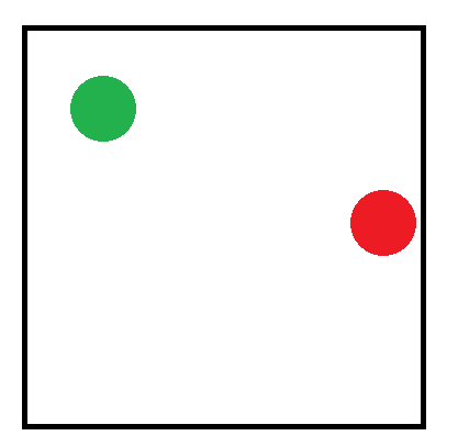
Let’s imagine the situation below where we are trying to find the distance between the red point and the green point:

One way to do this would be to pick one of the points (I’m picking red in this case) and clone it 8 times to surround the cell like the below. You’d calculate the distance from the green point to each of the 9 red points, and whatever distance was smallest would be the answer.

Something not so desirable about this is that it takes 9 distance calculations to find the minimum distance. You can work with squared distances instead of regular distances to avoid a square root on each of these distance calculations, but that’s still a bit of calculation to do.

Going up in dimensions makes the problem even worse. In 3D, it requires 27 distance calculations to find the shortest point, and 81 distance calculations in 4D!

Luckily there’s a better way to approach this.

Let’s say that our universe (image) is 1 unit by 1 unit big (aka we are working in texture UVs). If you look at the image with 9 copies of the red dot, you can see that they are just the 9 possible combinations of having -1, +0, +1 on each axis added to the red dot’s coordinates. All possible combinations of the x and y axis having -1, +0 or +1 added to them are valid locations of the red dot.

Looking at the distance formula we can see that if we minimize each axis individually, that we will also end up with the minimal distance overall.

d = \sqrt{(x_2-x_1)^2+(y_2-y_1)^2}

So, the better way is to minimize each axis individually.

On the x axis you’d find if the x axis distance between the red and green point is minimal when you subtract 1 from the red dot’s x axis position, leave it alone, or add 1.

Whichever x axis value of the red dot gives you the minimal x axis 1D distance is the x axis location to use.

You’d repeat for the y axis to get the y axis location to use (and would repeat for any further axes for higher dimensions).

This gives you the closest point which you can then plug into the distance formula to get the distance between the points in this wrap around space.

You can actually do better though.

Still working on each axis individually, you can calculate the absoluate value of the 1D distance between the two points on that axis. If that distance is greater than 0.5, the real distance for that axis is 1-distance.

The intuition here is that if you are in a 1d repeating space, if going from A to B is more than half the distance, it means that you went the wrong way, and that going the other way is shorter. The distance of that other way is one minus whatever distance you just calculated since the distance from one point to itself is 1!

Do that for each axis and use those 1d distances in the distance formula to get the actual distance.

This lets you minimize the distance without having to explicitly figure out which combination makes the point closest.

More importantly, it lets you efficiently calculate the distance between the two points in toroidal space (doughnut space!)

The computational complexity is a lot better. It’s now linear in the number of dimensions: O(N), instead of O(3^N).

Here is some C++ to show you how it would work in 2D.

float ToroidalDistance (float x1, float y1, float x2, float y2)
{
    float dx = std::abs(x2 - x1);
    float dy = std::abs(y2 - y1);

    if (dx > 0.5f)
        dx = 1.0f - dx;

    if (dy > 0.5f)
        dy = 1.0f - dy;

    return std::sqrt(dx*dx + dy*dy);
}

I hit this problem trying to make a tileable texture. I needed to place a few circles on a texture such that the circles weren’t too close to each other, even when the texture was tiled.

The calculations above gave me the basic tool needed to be able to calculate distances between points. Subtracting circle radii from the distance between points let me get toroidal distance between circles and make sure I didn’t place them too closely to each other.

That let me make an image that kept the distance constraints even when it was tiled.

Here’s an example image by itself:

Here is the image tiled:

Half Tile Offset Streaming World Grids

A number of years ago I worked on an open world game that got cancelled. Despite it not being released, I learned a few things.

If you try to make a game where the player can walk around a large world without loading screens, chances are that the whole world won’t fit in memory at once.

Since it can’t all fit in memory at once, as the player moves around you are going to have to unload old chunks of the world to make room for the new chunks that the player is about to enter.

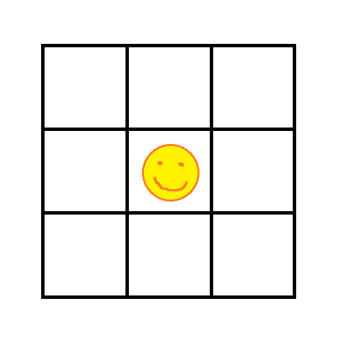
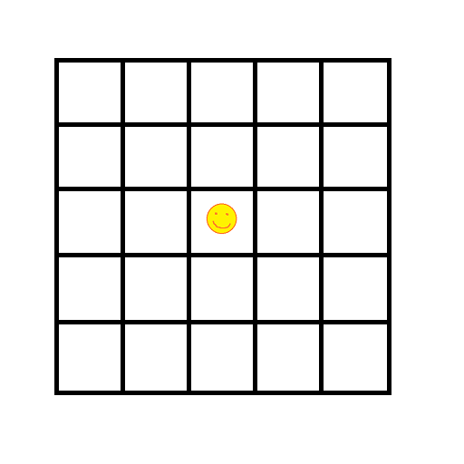
To simplify the problem, it’s really common to break the world up into a grid, and keep a radius of tiles loaded around the player at any one time.

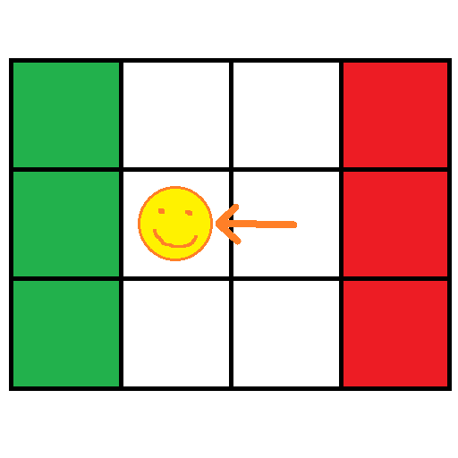
In the above you can see that 9 tiles are kept in memory. If the player crosses the boundary to the cell to the left, we unload the cells on the right (red cells) and load new cells in on the left (green cells).

The idea is that we keep a border of cells loaded around the player at all times so that they never see the edge of the world, but we don’t have to keep the whole world in memory at the same time.

The size of the cells can vary depending on the actual needs of your game. If you can travel very quickly in your game, you may need larger cells.

Instead of just having 9 large cells loaded at any one time, you may instead opt to have smaller cells but have more layers of them loaded at any one time. The below has 2 layers of cells loaded around the player, so has to keep 5×5 = 25 cells loaded at any one time. This can give you more granularity if you need it.

The number of cells you have to keep in memory when keeping N layers of cells loaded around the player is (2N+1)^2.

1 layer means 9 cells, 2 layers mean 25 cells, 3 layers mean 49 cells, 4 layers mean 81 cells and so on.

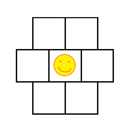
This isn’t the only way to arrange your world tiles though. You can also make it so every row of tiles is offset by half a tile from the one above it. That gives you a setup like this:

With this setup, keeping a single layer of cells loaded around the player takes only 7 cells instead of 9. That might not sound like much, but that means that your memory budget is 129% of what it was the other way.

Alternately, it means you can keep your cells at the same quality level but only have to load 78% as much stuff from disk as the player moves around the world.

For keeping N layers of cells around the player you need to keep 3N^2+3N+1 cells in memory.

1 layer means 7 cells, 2 layers mean 19 cells, 3 layers mean 37 cells, 4 layers mean 61 cells.

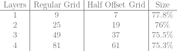
Here’s a table to show you how the regular grid compares to the half offset grid for cell counts. The savings do get better with more layers, but not very quickly.

\begin{array}{c|c|c|c} \text{Layers} & \text{Regular Grid} & \text{Half Offset Grid} & \text{Size} \\ \hline 1 & 9 & 7 & 77.8\%\\ 2 & 25 & 19 & 76\%\\ 3 & 49 & 37 & 75.5\%\\ 4 & 81 & 61 & 75.3\%\\ \end{array}

Overall, this is a pretty cool technique that is pretty low cost if you do this early in the project. Once you have a lot of content divided into a regular grid, it can be a challenge to move over to this half tile offset grid.

Some Notes From Readers

@chrispewebb said that an issue he’s faced when going this method is having T junctions on LODed terrain, but that skirts should be able to help there.

@runevision pointed out that while the memory requirements are lowered, so is the shortest distance (radius) from the player to data that isn’t loaded. One idea to deal with this if it’s a problem could be to use smaller cell sizes and to do more layers to make up for it.

Generating Random Numbers From a Specific Distribution With Rejection Sampling

The last post showed how to transform uniformly generated random numbers into any random number distribution you desired.

It did so by turning the PDF (probability density function) into a CDF (cumulative density function) and then inverting it – either analytically (making a function) or numerically (making a look up table).

This post will show you how to generate numbers from a PDF as well, but will do so using rejection sampling.

Dice

Let’s say you wanted to simulate a fair five sided die but that you only had a six sided die.

You can use rejection sampling for this by rolling a six sided die and ignoring the roll any time a six came up. Doing that, you do in fact get a fair five sided die roll!

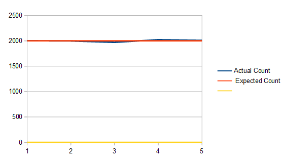
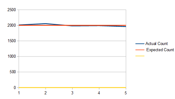
This shows doing that to get 10,000 five sided die rolls:

One disadvantage to this method is that you are throwing away die rolls which can be a source of inefficiency. In this setup it takes 1.2 six sided die rolls on average to get a valid five sided die roll since a roll will be thrown away 1/6 of the time.

Another disadvantage is that each time you need a new value, there are an unknown number of die rolls needed to get it. On average it’s true that you only need 1.2 die rolls, but in reality, it’s possible you may roll 10 sixes in a row. Heck it’s even technically possible (but very unlikely) that you could be rolling dice until the end of time and keep getting sixes. (Using PRNG’s in computers, this won’t happen, but it does take a variable number of rolls).

This is just to say: there is uneven and unpredictable execution time of this algorithm, and it needs an unknown (but somewhat predictable) amount of random numbers to work. This is true of the other forms of sampling methods I talk about lower down as well.

Instead of using a six sided die you could use a die of any size that is greater than (or equal to…) five. Here shows a twenty sided die simulating a five sided die:

It looks basically the same as using a six sided die, which makes sense (that shows that it works), but in this case, it actually took 4 rolls on average to make a valid five sided die roll, since the roll fails 15/20 times (3 out of 4 rolls will fail).

Quick Asides:

  • If straying from rejection sampling ideas for a minute, in the case of the twenty sided die, you could use modulus to get a fair five sided die roll each time: ((roll - 1) \% 5) + 1. This works because there is no remainder for 20 % 5. If there was a remainder it would bias the rolls towards the numbers <= the remainder, making them more likely to come up than the other numbers.

  • You could also get a four sided die roll at the same time if you didn’t want to waste any of this precious random information: ((roll - 1) / 5) + 1
  • Another algorithm to check out for discrete (integer) weighted random numbers is Vose’s method: Vose’s Method.

Box Around PDF

Moving back into the world of continuous valued random numbers and PDF’s, a simple version of how rejection sampling can be used is like this:

  1. Graph your PDF
  2. Draw a box around the PDF
  3. Generate a (uniform) random point in that box
  4. If the point is under the curve of the PDF, use the x axis value as your random number, else throw it out and go to 1

That’s all there is to it!

This works because the x axis value of your 2d point is the random number you might be choosing. The y axis value of your 2d point is a probability of choosing that point. Since the PDF graph is higher in places that are more probable, those places are more likely to accept your 2d point than places that have lower PDF values.

Furthermore, the average number of rejected samples vs accepted samples is based on the area under the PDF compared to the area of the box.

The number of samples on average will be the area of the box divided by the area of the PDF.

Since PDF’s by definition have to integrate to 1, that means that you are dividing by 1. So, to simplify: The number of samples on average will be the same as the area of the box!

If it’s hard to come up with the exact size of the box for the PDF, the box doesn’t have to fit exactly, but of course the tighter you can fit the box around the PDF, the fewer rejected samples you’ll have.

You don’t actually need to graph the PDF and draw a box to do this though. Just generate a 2d random number (a random x and a random y) and reject the point if PDF(x) < y.

Here I'm using this technique with the PDF y=2x where x is in [0,1) and I'm using a box that goes from (0,0) to (1,2) to get 100,000 samples.
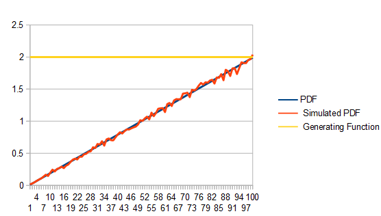
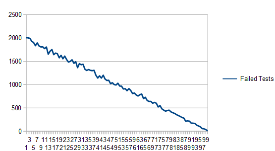
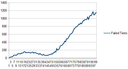
As expected, it took on average 2 points to get a single valid point since the area of the box is 2. Here are how many failed tests each histogram bucket had. Unsurprisingly, lower values of the PDF have more failed tests!

Moving to a more complex PDF, let’s look at y=\frac{x^3-10x^2+5x+11}{10.417}

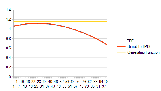
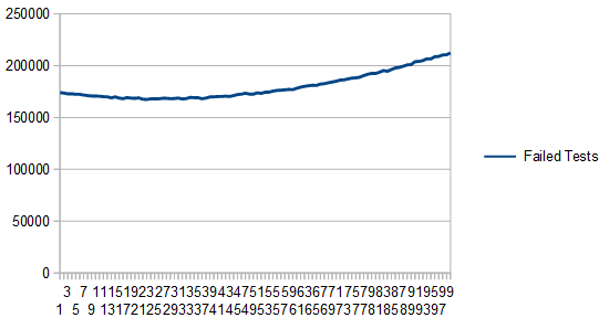
Here are 10 million samples (lots of samples to minimize the noise), using a box height of 1.2, which unsurprisingly takes 1.2 samples on average to get a valid sample:

Here is the graph of the failure counts:

Here the box has a height of 2.8. It still works, but uses 2.8 samples on average which is less efficient:

Here’s the graph of failure counts:

Something interesting about this technique is that technically, the distribution you are sampling from doesn’t even have to be a PDF! If you have negative parts of the graph, they will be treated as zero, assuming your box has a minimum y of 0. Also, the fact that your function may not integrate to (have an area of) 1 doesn’t matter at all.

Here we take the PDF from the last examples, and take off the division by a constant, so that it doesn’t integrate to 1: y=x^3-10x^2+5x+11

The interesting thing is that we get as output a normalized PDF (the red line), even though the distribution we were using to sample was not normalized (the blue line, which is mostly hidden behind the yellow line).

Here are the rejection counts:

Generating One PDF from Another PDF

In the last section we showed how to enclose a PDF in a box, make uniformly random 2d points, and use them to generate points from the PDF.

By enclosing it in a box, all we were really doing is putting it under a uniform distribition that was scaled up to be larger than the PDF at all points.

Now here’s the interesting thing: We aren’t limited to using the uniform distribution!

To generalize this technique, if you are trying to sample from a PDF f(x), you can use any PDF g(x) to do so, so long as you multiply g(x) by a scalar value M so that M*g(x)>= f(x) for all values of x. In other words: scale up g so that it’s always bigger than f.

Using this more generalized technique has one or two more steps than the other way, but allows for a tighter fit of a generating function, resulting in fewer samples thrown away.

Here’s how to do it:

  1. Generate a random number from the distribution g, and call it x.
  2. Calculate the percentage chance of x being chosen by getting a ratio of how likely that number is to be chosen in each PDF: \frac{f(x)}{M*g(x)}
  3. Generate a uniform random number from 0 to 1. If it’s less than the value you just calculated, accept x as the random number, else reject it and go back to 1.

Let’s see this in action!

We’ll generate numbers in a Gaussian distribution with a mean of 15 and a standard deviation of 5. We’ll truncate it to +/- 3 standard deviations so we want to generate random numbers from [0,30).

To generate these numbers, we’ll draw random numbers from the PDF y=x*0.002222. We’ll use an M value of 3 to scale up this PDF to always be greater than the Gaussian one.

Here is how it looks doing this with 20,000 samples:

We generate random numbers along the red line, multiply them by 3 to make them be the yellow line. Then, at whatever point we are at on the x axis, we divide the blue line value by the yellow line value and use that as an acceptance probability. Doing this and counting numbers in a histogram gives us our result – the green line. Since the end goal is the blue line, you can see it is indeed working! With a larger number of samples, the green line would more closely match the blue line.

Here’s the graph of the failed tests:

We have to take on average 3 samples before we get a valid random number. That shouldn’t be too surprising because both PDF’s start with area of 1, but we are multiplying one of them by 3 to make it always be larger than the other.

Something else interesting you might notice is that we have a lot fewer failed tests where the two PDF functions are more similar.

That is the power of this technique: If you can cheaply and easily generate samples that are “pretty close” to a harder distribution to sample from, you can use this technique to more cheaply sample from it.

Something to note is that just like in the last section, the target PDF doesn’t necessarily need to be a real PDF with only positive values and integrating to 1. It would work just the same with a non PDF function, just so long as the PDF generating the random numbers you start with is always above the function.

Some Other Notes

There is family of techniques called “adaptive rejection sampling” that will change the PDF they are drawing from whenever there is a failed test.

Basically, if you imagine the PDF you are drawing from as being a bunch of line segments connected together, you could imagine that whenever you failed a test, you moved a line segment down to be closer to the curve, so that when you sampled from that area again, the chances would be lower that you’d fail the test again.

Taking this to the limit, your sampling PDF will eventually become the PDF you are trying to sample from, and then using this PDF will be a no-op.

These techniques are a continued area of research.

Something else to note is that rejection sampling can be used to find random points within shapes.

For instance, a random point on a triangle, ellipse or circle could be done by putting a (tight) bounding box around the shape, generating points randomly in that box, and only accepting ones within the inner shape.

This can be extended to 3d shapes as well.

Some shapes have better ways to generate points within them that don’t involve iteration and rejected samples, but if all else fails, rejection sampling does indeed work!

At some point in the future I’d like to look into “Markov Chain Monte Carlo” more deeply. It seems like a very interesting technique to approach this same problem, but I have no idea if it’s used often in graphics, especially real time graphics.

Code

Here is the code that generated all the data from this post. The data was visualized with open office.

#define _CRT_SECURE_NO_WARNINGS
 
#include <stdio.h>
#include <random>
#include <array>
#include <unordered_map>

template <size_t NUM_TEST_SAMPLES, size_t SIMULATED_DICE_SIDES, size_t ACTUAL_DICE_SIDES>
void TestDice (const char* fileName)
{
    // seed the random number generator
    std::random_device rd;
    std::mt19937 rng(rd());
    std::uniform_int_distribution<size_t> dist(0, ACTUAL_DICE_SIDES-1);

    // generate the histogram
    std::array<size_t, SIMULATED_DICE_SIDES> histogram = { 0 };
    size_t rejectedSamples = 0;
    for (size_t i = 0; i < NUM_TEST_SAMPLES; ++i)
    {
        size_t roll = dist(rng);
        while (roll >= SIMULATED_DICE_SIDES)
        {
            ++rejectedSamples;
            roll = dist(rng);
        }
        histogram[roll]++;
    }

    // write the histogram and rejected sample count to a csv
    // an extra 0 data point forces the graph to include 0 in the scale. hack to make the data not look noisier than it really is.
    FILE *file = fopen(fileName, "w+t");
    fprintf(file, "Actual Count, Expected Count, , %0.2f samples needed per roll on average.\n", (float(NUM_TEST_SAMPLES) + float(rejectedSamples)) / float(NUM_TEST_SAMPLES));
    for (size_t value : histogram)
        fprintf(file, "%zu,%zu,0\n", value, (size_t)(float(NUM_TEST_SAMPLES) / float(SIMULATED_DICE_SIDES)));
    fclose(file);
}
 
template <size_t NUM_TEST_SAMPLES, size_t NUM_HISTOGRAM_BUCKETS, typename PDF_LAMBDA>
void Test (const char* fileName, float maxPDFValue, const PDF_LAMBDA& PDF)
{
    // seed the random number generator
    std::random_device rd;
    std::mt19937 rng(rd());
    std::uniform_real_distribution<float> dist(0.0f, 1.0f);
 
    // generate the histogram
    std::array<size_t, NUM_HISTOGRAM_BUCKETS> histogram = { 0 };
    std::array<size_t, NUM_HISTOGRAM_BUCKETS> failedTestCounts = { 0 };
    size_t rejectedSamples = 0;
    for (size_t i = 0; i < NUM_TEST_SAMPLES; ++i)
    {
        // Generate a sample from the PDF by generating a random 2d point.
        // If the y axis of the value is <= the value returned by PDF(x), accept it, else reject it.
        // NOTE: this takes an unknown number of iterations, and technically may NEVER finish.
        float pointX = 0.0f;
        float pointY = 0.0f;
        bool validPoint = false;
        while (!validPoint)
        {
            pointX = dist(rng);
            pointY = dist(rng) * maxPDFValue;
            float pdfValue = PDF(pointX);
            validPoint = (pointY <= pdfValue);

            // track number of failed tests per histogram bucket
            if (!validPoint)
            {
                size_t bin = (size_t)std::floor(pointX * float(NUM_HISTOGRAM_BUCKETS));
                failedTestCounts[std::min(bin, NUM_HISTOGRAM_BUCKETS - 1)]++;
                ++rejectedSamples;
            }
        }
 
        // increment the correct bin in the histogram
        size_t bin = (size_t)std::floor(pointX * float(NUM_HISTOGRAM_BUCKETS));
        histogram[std::min(bin, NUM_HISTOGRAM_BUCKETS -1)]++;
    }
 
    // write the histogram and pdf sample to a csv
    FILE *file = fopen(fileName, "w+t");
    fprintf(file, "PDF, Simulated PDF, Generating Function, Failed Tests, %0.2f samples needed per value on average.\n", (float(NUM_TEST_SAMPLES) + float(rejectedSamples)) / float(NUM_TEST_SAMPLES));
    for (size_t i = 0; i < NUM_HISTOGRAM_BUCKETS; ++i)
    {
        float x = (float(i) + 0.5f) / float(NUM_HISTOGRAM_BUCKETS);
        float pdfSample = PDF(x);
        fprintf(file, "%f,%f,%f,%f\n",
            pdfSample,
            NUM_HISTOGRAM_BUCKETS * float(histogram[i]) / float(NUM_TEST_SAMPLES),
            maxPDFValue,
            float(failedTestCounts[i])
        );
    }
    fclose(file);
}

template <size_t NUM_TEST_SAMPLES, size_t NUM_HISTOGRAM_BUCKETS, typename PDF_LAMBDA>
void TestNotPDF (const char* fileName, float maxPDFValue, float normalizationConstant, const PDF_LAMBDA& PDF)
{
    // seed the random number generator
    std::random_device rd;
    std::mt19937 rng(rd());
    std::uniform_real_distribution<float> dist(0.0f, 1.0f);
 
    // generate the histogram
    std::array<size_t, NUM_HISTOGRAM_BUCKETS> histogram = { 0 };
    std::array<size_t, NUM_HISTOGRAM_BUCKETS> failedTestCounts = { 0 };
    size_t rejectedSamples = 0;
    for (size_t i = 0; i < NUM_TEST_SAMPLES; ++i)
    {
        // Generate a sample from the PDF by generating a random 2d point.
        // If the y axis of the value is <= the value returned by PDF(x), accept it, else reject it.
        // NOTE: this takes an unknown number of iterations, and technically may NEVER finish.
        float pointX = 0.0f;
        float pointY = 0.0f;
        bool validPoint = false;
        while (!validPoint)
        {
            pointX = dist(rng);
            pointY = dist(rng) * maxPDFValue;
            float pdfValue = PDF(pointX);
            validPoint = (pointY <= pdfValue);

            // track number of failed tests per histogram bucket
            if (!validPoint)
            {
                size_t bin = (size_t)std::floor(pointX * float(NUM_HISTOGRAM_BUCKETS));
                failedTestCounts[std::min(bin, NUM_HISTOGRAM_BUCKETS - 1)]++;
                ++rejectedSamples;
            }
        }
 
        // increment the correct bin in the histogram
        size_t bin = (size_t)std::floor(pointX * float(NUM_HISTOGRAM_BUCKETS));
        histogram[std::min(bin, NUM_HISTOGRAM_BUCKETS -1)]++;
    }
 
    // write the histogram and pdf sample to a csv
    FILE *file = fopen(fileName, "w+t");
    fprintf(file, "Function, Simulated PDF, Scaled Simulated PDF, Generating Function, Failed Tests, %0.2f samples needed per value on average.\n", (float(NUM_TEST_SAMPLES) + float(rejectedSamples)) / float(NUM_TEST_SAMPLES));
    for (size_t i = 0; i < NUM_HISTOGRAM_BUCKETS; ++i)
    {
        float x = (float(i) + 0.5f) / float(NUM_HISTOGRAM_BUCKETS);
        float pdfSample = PDF(x);
        fprintf(file, "%f,%f,%f,%f,%f\n",
            pdfSample,
            NUM_HISTOGRAM_BUCKETS * float(histogram[i]) / float(NUM_TEST_SAMPLES),
            NUM_HISTOGRAM_BUCKETS * float(histogram[i]) / float(NUM_TEST_SAMPLES) * normalizationConstant,
            maxPDFValue,
            float(failedTestCounts[i])
        );
    }
    fclose(file);
}

template <size_t NUM_TEST_SAMPLES, size_t NUM_HISTOGRAM_BUCKETS, typename PDF_F_LAMBDA, typename PDF_G_LAMBDA, typename INVERSE_CDF_G_LAMBDA>
void TestPDFToPDF (const char* fileName, const PDF_F_LAMBDA& PDF_F, const PDF_G_LAMBDA& PDF_G, float M, const INVERSE_CDF_G_LAMBDA& Inverse_CDF_G, float rngRange)
{
    // We generate a sample from PDF F by generating a sample from PDF G, and accepting it with probability PDF_F(x)/(M*PDF_G(x))

    // seed the random number generator
    std::random_device rd;
    std::mt19937 rng(rd());
    std::uniform_real_distribution<float> dist(0.0f, 1.0f);
 
    // generate the histogram
    std::array<size_t, NUM_HISTOGRAM_BUCKETS> histogram = { 0 };
    std::array<size_t, NUM_HISTOGRAM_BUCKETS> failedTestCounts = { 0 };
    size_t rejectedSamples = 0;
    for (size_t i = 0; i < NUM_TEST_SAMPLES; ++i)
    {
        // generate random points until we have one that's accepted
        // NOTE: this takes an unknown number of iterations, and technically may NEVER finish.
        float sampleG = 0.0f;
        bool validPoint = false;
        while (!validPoint)
        {
            // Generate a sample from the soure PDF G
            sampleG = Inverse_CDF_G(dist(rng));

            // calculate the ratio of how likely we are to accept this sample
            float acceptChance = PDF_F(sampleG) / (M * PDF_G(sampleG));

            // see if we should accept it
            validPoint = dist(rng) <= acceptChance;

            // track number of failed tests per histogram bucket
            if (!validPoint)
            {
                size_t bin = (size_t)std::floor(sampleG * float(NUM_HISTOGRAM_BUCKETS) / rngRange);
                failedTestCounts[std::min(bin, NUM_HISTOGRAM_BUCKETS - 1)]++;
                ++rejectedSamples;
            }
        }

        // increment the correct bin in the histogram
        size_t bin = (size_t)std::floor(sampleG * float(NUM_HISTOGRAM_BUCKETS) / rngRange);
        histogram[std::min(bin, NUM_HISTOGRAM_BUCKETS - 1)]++;
    }
 
    // write the histogram and pdf sample to a csv
    FILE *file = fopen(fileName, "w+t");
    fprintf(file, "PDF F,PDF G,Scaled PDF G,Simulated PDF,Failed Tests,%0.2f samples needed per value on average.\n", (float(NUM_TEST_SAMPLES) + float(rejectedSamples)) / float(NUM_TEST_SAMPLES));
    for (size_t i = 0; i < NUM_HISTOGRAM_BUCKETS; ++i)
    {
        float x = (float(i) + 0.5f) * rngRange / float(NUM_HISTOGRAM_BUCKETS);
        
        fprintf(file, "%f,%f,%f,%f,%f\n",
            PDF_F(x),
            PDF_G(x),
            PDF_G(x)*M,
            NUM_HISTOGRAM_BUCKETS * float(histogram[i]) / (float(NUM_TEST_SAMPLES)*rngRange),
            float(failedTestCounts[i])
        );
    }
    fclose(file);
}
 
int main(int argc, char **argv)
{
    // Dice
    {
        // Simulate a 5 sided dice with a 6 sided dice
        TestDice<10000, 5, 6>("test1_5_6.csv");

        // Simulate a 5 sided dice with a 20 sided dice
        TestDice<10000, 5, 20>("test1_5_20.csv");
    }

    // PDF y=2x, simulated with a uniform distribution
    {
        auto PDF = [](float x) { return 2.0f * x; };

        Test<1000, 100>("test2_1k.csv", 2.0f, PDF);
        Test<100000, 100>("test2_100k.csv", 2.0f, PDF);
        Test<1000000, 100>("test2_1m.csv", 2.0f, PDF);
    }

    // PDF y=(x^3-10x^2+5x+11)/10.417, simulated with a uniform distribution
    {
        auto PDF = [](float x) {return (x*x*x - 10.0f*x*x + 5.0f*x + 11.0f) / (10.417f); };
        Test<10000000, 100>("test3_10m_1_15.csv", 1.15f, PDF);
        Test<10000000, 100>("test3_10m_1_5.csv", 1.5f, PDF);
        Test<10000000, 100>("test3_10m_2_8.csv", 2.8f, PDF);
    }

    // function (not PDF, Doesn't integrate to 1!) y=(x^3-10x^2+5x+11), simulated with a scaled up uniform distribution
    {
        auto PDF = [](float x) {return (x*x*x - 10.0f*x*x + 5.0f*x + 11.0f); };
        TestNotPDF<10000000, 100>("test4_10m_12_5.csv", 12.5f, 10.417f, PDF);
    }

    // Generate samples from PDF F using samples from PDF G.  random numbers are from 0 to 30.
    // F PDF = gaussian distribution, mean 15, std dev of 5.  Truncated to +/- 3 stddeviations.
    // G PDF = x*0.002222
    // G CDF = 0.001111 * x^2
    // G inverted CDF = (1000 * sqrt(x)) / sqrt(1111)
    // M = 3
    {
        // gaussian PDF F
        const float mean = 15.0f;
        const float stddev = 5.0f;
        auto PDF_F = [=] (float x) -> float
        {
            return (1.0f / (stddev * sqrt(2.0f * (float)std::_Pi))) * std::exp(-0.5f * pow((x - mean) / stddev, 2.0f));
        };

        // PDF G
        auto PDF_G = [](float x) -> float
        {
            return x * 0.002222f;
        };

        // Inverse CDF of G
        auto Inverse_CDF_G = [] (float x) -> float
        {
            return 1000.0f * std::sqrtf(x) / std::sqrtf(1111.0f);
        };

        TestPDFToPDF<20000, 100>("test5.csv", PDF_F, PDF_G, 3.0f, Inverse_CDF_G, 30.0f);
    }

    return 0;
}

Generating Random Numbers From a Specific Distribution By Inverting the CDF

The last post talked about the normal distribution and showed how to generate random numbers from that distribution by generating regular (uniform) random numbers and then counting the bits.

What would you do if you wanted to generate random numbers from a different, arbitrary distribution though? Let’s say the distribution is defined by a function even.

It turns out that in general this is a hard problem, but in practice there are a few ways to approach it. The below are the most common techniques for achieving this that I’ve seen.

  • Inverting the CDF (analytically or numerically)
  • Rejection Sampling
  • Markov Chain Monte Carlo
  • Ziggurat algorithm

This post talks about the first one listed: Inverting the CDF.

What Is A CDF?

The last post briefly explained that a PDF is a probability density function and that it describes the relative probability of numbers being chosen at random. A requirement of a PDF is that it has non negative value everywhere and also that the area under the curve is 1.

It needs to be non negative everywhere because a negative probability doesn’t make any sense. It needs to have an area under the curve of 1 because that means it represents the full 100% probability of all possible outcomes.

CDF stands for “Cumulative distribution function” and is related to the PDF.

A PDF is a function y=f(x) where y is the probability of the number x number being chosen at random from the distribution.

A CDF is a function y=f(x) where y is the probability of the number x, or any lower number, being chosen at random from that distribution.

You get a CDF from a PDF by integrating the PDF. From there you make sure that the CDF has a starting y value of 0, and an ending value of 1. You might have to do a bias (addition or subtraction) and/or scale (multiplication or division) to make that happen.

Why Invert the CDF? (And Not the PDF?)

With both a PDF and a CDF, you plug in a number, and you get information about probabilities relating to that number.

To get a random number from a specific distribution, we want to do the opposite. We want to plug in a probability and get out the number corresponding to that probability.

Basically, we want to flip x and y in the equation and solve for y, so that we have a function that does this. That is what we have to do to invert the CDF.

Why invert the CDF though and not the PDF? Check out the images below from Wikipedia. The first is some Gaussian PDF’s and the second is the same distributions as CDF’s:


The issue is that if we flip x and y’s in a PDF, there would be multiple y values corresponding to the same x. This isn’t true in a CDF.

Let’s work through sampling some PDFs by inverting the CDF.

Example 0: y=1

This is the easiest case and represents uniform random numbers, where every number is evenly likely to be chosen.

Our PDF equation is: y=1 where x \in [0,1]. The graph looks like this:

If we integrate the pdf to get the cdf, we get y=x where x \in [0,1] which looks like this:

Now, to invert the cdf, we flip x and y, and then solve for y again. It’s trivially easy…

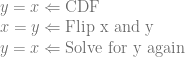
y=x \Leftarrow \text{CDF}\\ x=y \Leftarrow \text{Flip x and y}\\ y=x \Leftarrow \text{Solve for y again}

Now that we have our inverted CDF, which is y=x, we can generate uniform random numbers, plug them into that equation as x and get y which is the actual value drawn from our PDF.

You can see that since we are plugging in numbers from an even distribution and not doing anything to them at all, that the result is going to an even distribution as well. So, we are in fact generating uniformly distributed random numbers using this inverted CDF, just like our PDF asked for.

This is so trivially simple it might be confusing. If so, don’t sweat it. Move onto the next example and you can come back to this later if you want to understand what I’m talking about here.

Note: The rest of the examples are going to have x in [0,1] as well but we are going to stop explicitly saying so. This process still works when x is in a different range of values, but for simplicity we’ll just have x be in [0,1] for the rest of the post.

Example 1: y=2x

The next easiest case for a PDF is y=2x which looks like this:

You might wonder why it’s y=2x instead of y=x. This is because the area under the curve y=x is 0.5. PDF’s need to have an area of 1, so I multiplied by 2 to make it have an area of 1.

What this PDF means is that small numbers are less likely to be picked than large numbers.

If we integrate the PDF y=2x to get the CDF, we get y=x^2 which looks like this:

Now let’s flip x and y and solve for y again.

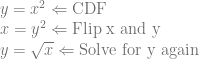
y=x^2 \Leftarrow \text{CDF}\\ x=y^2 \Leftarrow \text{Flip x and y}\\ y=\sqrt{x} \Leftarrow \text{Solve for y again}

We now have our inverted CDF which is y=\sqrt{x} and looks like this:

Now, if we plug uniformly random numbers into that formula as x, we should get as output samples that follow the probability of our PDF.

We can use a histogram to see if this is really true. We can generate some random numbers, square root them, and count how many are in each range of values.

Here is a histogram where I took 1,000 random numbers, square rooted them, and put their counts into 100 buckets. Bucket 1 counted how many numbers were in [0, 0.01), bucket 2 counted how many numbers were in [0.01, 0.02) and so on until bucket 100 which counted how many numbers were in [0.99, 1.0).

Increasing the number of samples to 100,000 it gets closer:

At 1,000,000 samples you can barely see a difference:

The reason it doesn’t match up at lower sample counts is just due to the nature of random numbers being random. It does match up, but you’ll have some variation with lower sample counts.

Example 2: y=3x^2

Let’s check out the PDF y=3x^2. The area under that curve where x is in [0,1) is 1.0 and it’s non negative everywhere in that range too, so it’s a valid PDF.

Integrating that, we get y=x^3 for the CDF. Then we invert the CDF:

y=x^3 \Leftarrow \text{CDF}\\ x=y^3 \Leftarrow \text{Flip x and y}\\ y=\sqrt[3]{x} \Leftarrow \text{Solve for y again}

And here is a 100,000 sample histogram vs the PDF to verify that we got the right answer:

Example 3: Numeric Solution

So far we’ve been able to invert the CDF to get a nice easy function to transform uniform distribution random numbers into numbers from the distribution described by the PDF.

Sometimes though, inverting a CDF isn’t possible, or gives a complex equation that is costly to evaluate. In these cases, you can actually invert the CDF numerically via a lookup table.

A lookup table may also be desired in cases where eg you have a pixel shader that is drawing numbers from a PDF, and instead of making N shaders for N different PDFs, you want to unify them all into a single shader. Passing a lookup table via a constant buffer, or perhaps even via a texture can be a decent solution here. (Note: if storing in a texture you may be interested in fitting the data with curves and using this technique to store it and recall it from the texture: GPU Texture Sampler Bezier Curve Evaluation)

Let’s invert a PDF numerically using a look up table to see how that would work.

Our PDF will be:

y=\frac{x^3-10x^2+5x+11}{10.417}

And looks like this:

It’s non negative in the range we care about and it integrates to 1.0 – or it integrates closely enough… the division by 10.417 is there for that reason, and using more digits would get it closer to 1.0.

What we are going to do is evaluate that PDF at N points to get a probability for those samples of numbers. That will give us a lookup table for our PDF.

We are then going to make each point be the sum of all the PDF samples to the left of it to make a lookup table for a CDF. We’ll also have to normalize the CDF table since it’s likely that our PDF samples don’t all add up (integrate) to 1.0. We do this by dividing every item in the CDF by the last entry in the CDF. If you look at the table after that, it will fully cover everything from 0% to 100% probability.

Below are some histogram comparisons of the lookup table technique vs the actual PDF.

Here is 100 million samples (to make it easier to see the data without very much random noise), in 100 histogram buckets, and a lookup table size of 3 which is pretty low quality:

Increasing it to a lookup table of size 5 gives you this:

Here’s 10:

25:

And here’s 100:

So, not surprisingly, the size of the lookup table affects the quality of the results!

Code

here is the code I used to generate the data in this post, which i visualized with open office. I visualized the function graphs using wolfram alpha.

#define _CRT_SECURE_NO_WARNINGS

#include 
#include 
#include 
#include 

template 
void Test (const char* fileName, const PDF_LAMBDA& PDF, const INVERSE_CDF_LAMBDA& inverseCDF)
{
    // seed the random number generator
    std::random_device rd;
    std::mt19937 rng(rd());
    std::uniform_real_distribution dist(0.0f, 1.0f);

    // generate the histogram
    std::array histogram = { 0 };
    for (size_t i = 0; i < NUM_TEST_SAMPLES; ++i)
    {
        // put a uniform random number into the inverted CDF to sample the PDF
        float x = dist(rng);
        float y = inverseCDF(x);

        // increment the correct bin on the histogram
        size_t bin = (size_t)std::floor(y * float(NUM_HISTOGRAM_BUCKETS));
        histogram[std::min(bin, NUM_HISTOGRAM_BUCKETS -1)]++;
    }

    // write the histogram and pdf sample to a csv
    FILE *file = fopen(fileName, "w+t");
    fprintf(file, "PDF, Inverted CDF\n");
    for (size_t i = 0; i < NUM_HISTOGRAM_BUCKETS; ++i)
    {
        float x = (float(i) + 0.5f) / float(NUM_HISTOGRAM_BUCKETS);
        float pdfSample = PDF(x);
        fprintf(file, "%f,%f\n",
            pdfSample,
            NUM_HISTOGRAM_BUCKETS * float(histogram[i]) / float(NUM_TEST_SAMPLES)
        );
    }
    fclose(file);
}

template 
void TestPDFOnly (const char* fileName, const PDF_LAMBDA& PDF)
{
    // make the CDF lookup table by sampling the PDF
    // NOTE: we could integrate the buckets by averaging multiple samples instead of just the 1. This bucket integration is pretty low tech and low quality.
    std::array CDFLookupTable;
    float value = 0.0f;
    for (size_t i = 0; i < LOOKUP_TABLE_SIZE; ++i)
    {
        float x = float(i) / float(LOOKUP_TABLE_SIZE - 1); // The -1 is so we cover the full range from 0% to 100%
        value += PDF(x);
        CDFLookupTable[i] = value;
    }

    // normalize the CDF - make sure we span the probability range 0 to 1.
    for (float& f : CDFLookupTable)
        f /= value;

    // make our LUT based inverse CDF
    // We will binary search over the y's (which are sorted smallest to largest) looking for the x, which is implied by the index.
    // I'm sure there's a better & more clever lookup table setup for this situation but this should give you an idea of the technique
    auto inverseCDF = [&CDFLookupTable] (float y) {

        // there is an implicit entry of "0%" at index -1
        if (y < CDFLookupTable[0])
        {
            float t = y / CDFLookupTable[0];
            return t / float(LOOKUP_TABLE_SIZE);
        }

        // get the lower bound in the lut using a binary search
        auto it = std::lower_bound(CDFLookupTable.begin(), CDFLookupTable.end(), y);

        // figure out where we are at in the table
        size_t index = it - CDFLookupTable.begin();

        // Linearly interpolate between the values
        // NOTE: could do other interpolation methods, like perhaps cubic (https://blog.demofox.org/2015/08/08/cubic-hermite-interpolation/)
        float t = (y - CDFLookupTable[index - 1]) / (CDFLookupTable[index] - CDFLookupTable[index - 1]);
        float fractionalIndex = float(index) + t;
        return fractionalIndex / float(LOOKUP_TABLE_SIZE);
    };

    // call the usual function to do the testing
    Test(fileName, PDF, inverseCDF);
}

int main (int argc, char **argv)
{
    // PDF: y=2x
    // inverse CDF: y=sqrt(x)
    {
        auto PDF = [] (float x) { return 2.0f * x; };
        auto inverseCDF = [] (float x) { return std::sqrt(x); };

        Test("test1_1k.csv", PDF, inverseCDF);
        Test("test1_100k.csv", PDF, inverseCDF);
        Test("test1_1m.csv", PDF, inverseCDF);
    }

    // PDF: y=3x^2
    // inverse CDF: y=cuberoot(x) aka y = pow(x, 1/3)
    {
        auto PDF = [] (float x) { return 3.0f * x * x; };
        auto inverseCDF = [](float x) { return std::pow(x, 1.0f / 3.0f); };

        Test("test2_100k.csv", PDF, inverseCDF);
    }

    // PDF: y=(x^3-10x^2+5x+11)/10.417
    // Inverse CDF Numerically via a lookup table
    {
        auto PDF = [] (float x) {return (x*x*x - 10.0f*x*x + 5.0f*x + 11.0f) / (10.417f); };
        TestPDFOnly("test3_100m_3.csv", PDF);
        TestPDFOnly("test3_100m_5.csv", PDF);
        TestPDFOnly("test3_100m_10.csv", PDF);
        TestPDFOnly("test3_100m_25.csv", PDF);
        TestPDFOnly("test3_100m_100.csv", PDF);
    }

    return 0;
}

Counting Bits & The Normal Distribution

I recently saw some interesting posts on twitter about the normal distribution:

I’m not really a statistics kind of guy, but knowing that probability distributions come up in graphics (Like in PBR & Path Tracing), it seemed like a good time to upgrade knowledge in this area while sharing an interesting technique for generating normal distribution random numbers.

Basics

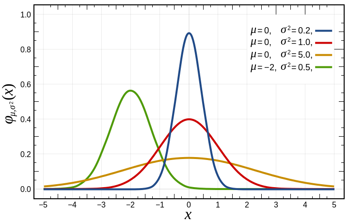
Below is an image showing a few normal (aka Gaussian) distributions (from wikipedia).

Normal distributions are defined by these parameters:

  • \mu – “mu” is the mean. This is the average value of the distribution. This is where the center (peak) of the curve is on the x axis.
  • \sigma^2 – “sigma squared” is the variance, and is just the standard deviation squared. I find standard deviation more intuitive to think about.
  • \sigma – “sigma” is the standard deviation, which (surprise surprise!) is the square root of the variance. This controls the “width” of the graph. The area under the cover is 1.0, so as you increase standard deviation and make the graph wider, it also gets shorter.
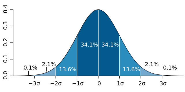
Here’s a diagram of standard deviations to help understand them (also from wikipedia):

I find the standard deviation intuitive because 68.2% of the data is within one standard deviation from the mean (on the plus and minus side of the mean). 95.4% of the data is within two standard deviations of the mean.

Standard deviation is given in the same units as the data itself, so if a bell curve described scores on a test, with a mean of 80 and a standard deviation of 5, it means that 68.2% of the students got between 75 and 85 points on the test, and that 95.4% of the students got between 70 and 90 points on the test.

The normal distribution is what’s called a “probability density function” or pdf, which means that the y axis of the graph describes the likelyhood of the number on the x axis being chosen at random.

This means that if you have a normal distribution that has a specific mean and variance (standard deviation), that numbers closer to the mean are more likely to be chosen randomly, while numbers farther away are less likely. The variance controls how the probability drops off as you get farther away from the mean.

Thinking about standard deviation again, 68.2% of the random numbers generated will be within 1 standard deviation of the mean (+1 std dev or -1 std dev). 95.4% will be within 2 standard deviations.

Generating Normal Distribution Random Numbers – Coin Flips

Generating uniform random numbers, where every number is as likely as every other number, is pretty simple. In the physical world, you can roll some dice or flip some coins. In the software world, you can use PRNGs.

How would you generate random numbers that follow a normal distribution though?

In C++, there is std::normal_distribution that can do this for you. There is also something called the Box-Muller transform that can turn uniformly distributed random numbers into normal distribution random numbers (info here: Generating Gaussian Random Numbers).

I want to talk about something else though and hopefully build some better intuition.

First let’s look at coin flips.

If you flip a fair coin a million times and keep a count of how many heads and tails you saw, you might get 500014 heads and 499986 tails (I got this with a PRNG – std::mt19937). That is a pretty uniform distribution of values in the range of [0,1]. (breadcrumb: pascal’s triangle row 2 is 1,1)

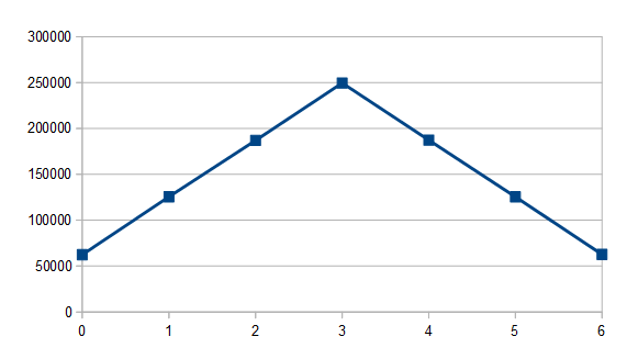
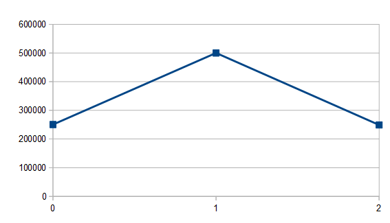
Let’s flip two coins at a time though and add our values together (say that heads is 0 and tails is 1). Here’s what that graph looks like:

Out of 1 million flips, 250639 had no tails, 500308 had one tail, and 249053 had two tails. It might seem weird that they aren’t all even, but it makes more sense when you look at the outcome of flipping two coins: we can get heads/heads (00), heads/tails (01), tails/heads (10) or tails/tails (11). Two of the four possibilities have a single tails, so it makes sense that flipping two coins and getting one coin being a tail would be twice as likely as getting no tails or two tails. (breadcrumb: pascal’s triangle row 3 is 1,2,1)

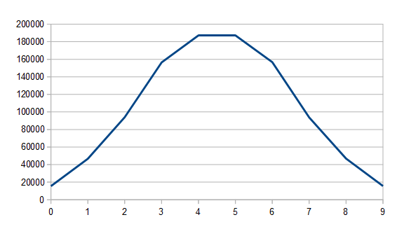
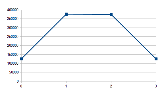
What happens when we sum 3 coins? With a million flips I got 125113 0’s, 375763 1’s, 373905 2’s and 125219 3’s.

If you work out the possible combinations, there is 1 way to get 0, 3 ways to get 1, 3 ways to get 2 and 1 way to get 3. Those numbers almost exactly follow that 1, 3, 3, 1 probability. (breadcrumb: pascal’s triangle row 4 is 1,3,3,1)

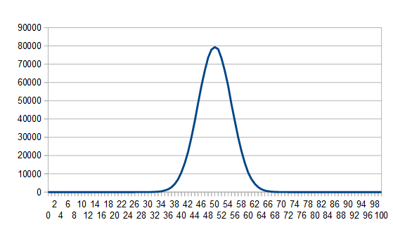
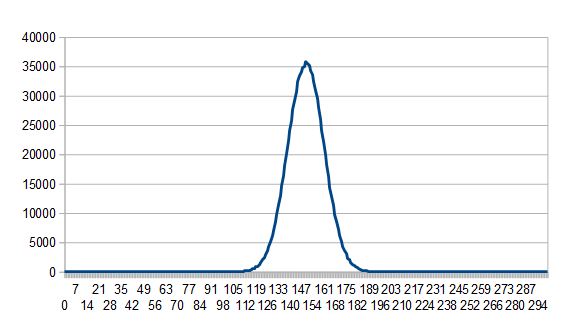
If we flip 100 coins and sum them, we get this:

That looks a bit like the normal distribution graphs at the beginning of this post doesn’t it?

Flipping and summing coins will get you something called the “Binomial Distribution”, and the interesting thing there is that the binomial distribution approaches the normal distribution the more coins you are summing together. At an infinite number of coins, it is the normal distribution.

Generating Normal Distribution Random Numbers – Dice Rolls

What if instead of flipping coins, we roll dice?

Well, rolling a 4 sided die a million times, you get each number roughly the same percentage of the time as you’d expect; roughly 25% each. 250125 0’s, 250103 1’s, 249700 2’s, 250072 3’s.

If we sum two 4 sided dice rolls we get this:

If we sum three 4 sided dice rolls we get this:

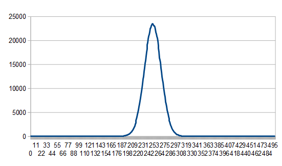
And if we sum one hundred we get this, which sure looks like a normal distribution:

This isn’t limited to four sided dice though, here’s one hundred 6 sided dice being summed:

With dice, instead of being a “binomial distribution”, it’s called a “multinomial distribution”, but as the number of dice goes to infinity, it also approaches the normal distribution.

This means you can get a normal distribution with not only coins, but any sided dice in general.

An even stronger statement than that is the Central Limit Theorem which says that if you have random numbers from ANY distribution, if you add enough of em together, you’ll often approach a normal distribution.

Strange huh?

Generating Normal Distribution Random Numbers – Counting Bits

Now comes a fun way of generating random numbers which follow a normal distribution. Are you ready for it?

Simply generate an N bit random number and return how many 1 bits are set.

That gives you a random number that follows a normal distribution!

One problem with this is that you have very low “resolution” random numbers. Counting the bits of a 64 bit random number for instance, you can only return 0 through 64 so there are only 65 possible random numbers.

That is a pretty big limitation, but if you need normal distribution numbers calculated quickly and don’t mind if they are low resolution (like in a pixel shader?), this technique could work well for you.

Another problem though is that you don’t have control over the variance or the mean of the distribution.

That isn’t a super huge deal though because you can easily convert numbers from one normal distribution into another normal distribution.

To do so, you get your normal distribution random number. First you subtract the mean of the distribution to make it centered on 0 (have a mean of 0). You then divide it by the standard deviation to make it be part of a distribution which has a standard deviation of 1.

At this point you have a random number from a normal distribution which has a mean of 0 and a standard deviation of 1.

Next, you multiply the number by the standard deviation of the distribution you want, and lastly you add the mean of the distribution you want.

That’s pretty simple (and is implemented in the source code at the bottom of this post), but to do this you need to know what standard deviation (variance) and mean you are starting with.

If you have some way to generate random numbers in [0, N) and you are summing M of those numbers together, the mean is M*(N-1)/2. Note that if you instead are generating random numbers in [1,N], the mean instead is M*(N+1)/2.

The variance in either case is M*(N^2-1)/12. The standard deviation is the square root of that.

Using that information you have everything you need to generate normal distribution random numbers of a specified mean and variance.

Thanks to @fahickman for the help on calculating mean and variance of dice roll sums.

Code

Here is the source code I used to generate the data which was used to generate the graphs in this post. There is also an implementation of the bit counting algorithm i mentioned, which converts to the desired mean and variance.

#define _CRT_SECURE_NO_WARNINGS

#include <array>
#include <random>
#include <stdint.h>
#include <stdio.h>
#include <limits>

const size_t c_maxNumSamples = 1000000;
const char* c_fileName = "results.csv";

template <size_t DiceRange, size_t DiceCount, size_t NumBuckets>
void DumpBucketCountsAddRandomNumbers (size_t numSamples, const std::array<size_t, NumBuckets>& bucketCounts)
{
    // open file for append if we can
    FILE* file = fopen(c_fileName, "a+t");
    if (!file)
        return;

    // write the info
    float mean = float(DiceCount) * float(DiceRange - 1.0f) / 2.0f;
    float variance = float(DiceCount) * (DiceRange * DiceRange) / 12.0f;
    if (numSamples == 1)
    {
        fprintf(file, "\"%zu random numbers [0,%zu) added together (sum %zud%zu). %zu buckets.  Mean = %0.2f.  Variance = %0.2f.  StdDev = %0.2f.\"\n", DiceCount, DiceRange, DiceCount, DiceRange, NumBuckets, mean, variance, std::sqrt(variance));
        fprintf(file, "\"\"");
        for (size_t i = 0; i < NumBuckets; ++i)
            fprintf(file, ",\"%zu\"", i);
        fprintf(file, "\n");
    }
    fprintf(file, "\"%zu samples\",", numSamples);

    // report the samples
    for (size_t count : bucketCounts)
        fprintf(file, "\"%zu\",", count);

    fprintf(file, "\"\"\n");
    if (numSamples == c_maxNumSamples)
        fprintf(file, "\n");

    // close file
    fclose(file);
}

template <size_t DiceSides, size_t DiceCount>
void AddRandomNumbersTest ()
{
    std::mt19937 rng;
    rng.seed(std::random_device()());
    std::uniform_int_distribution<size_t> dist(size_t(0), DiceSides - 1);

    std::array<size_t, (DiceSides - 1) * DiceCount + 1> bucketCounts = { 0 };

    size_t nextDump = 1;
    for (size_t i = 0; i < c_maxNumSamples; ++i)
    {
        size_t sum = 0;
        for (size_t j = 0; j < DiceCount; ++j)
            sum += dist(rng);

        bucketCounts[sum]++;

        if (i + 1 == nextDump)
        {
            DumpBucketCountsAddRandomNumbers<DiceSides, DiceCount>(nextDump, bucketCounts);
            nextDump *= 10;
        }
    }
}

template <size_t NumBuckets>
void DumpBucketCountsCountBits (size_t numSamples, const std::array<size_t, NumBuckets>& bucketCounts)
{
    // open file for append if we can
    FILE* file = fopen(c_fileName, "a+t");
    if (!file)
        return;

    // write the info
    float mean = float(NumBuckets-1) * 1.0f / 2.0f;
    float variance = float(NumBuckets-1) * 3.0f / 12.0f;
    if (numSamples == 1)
    {
        fprintf(file, "\"%zu random bits (coin flips) added together. %zu buckets.  Mean = %0.2f.  Variance = %0.2f.  StdDev = %0.2f.\"\n", NumBuckets - 1, NumBuckets, mean, variance, std::sqrt(variance));
        fprintf(file, "\"\"");
        for (size_t i = 0; i < NumBuckets; ++i)
            fprintf(file, ",\"%zu\"", i);
        fprintf(file, "\n");
    }
    fprintf(file, "\"%zu samples\",", numSamples);

    // report the samples
    for (size_t count : bucketCounts)
        fprintf(file, "\"%zu\",", count);

    fprintf(file, "\"\"\n");
    if (numSamples == c_maxNumSamples)
        fprintf(file, "\n");

    // close file
    fclose(file);
}

template <size_t NumBits> // aka NumCoinFlips!
void CountBitsTest ()
{

    size_t maxValue = 0;
    for (size_t i = 0; i < NumBits; ++i)
        maxValue = (maxValue << 1) | 1;

    std::mt19937 rng;
    rng.seed(std::random_device()());
    std::uniform_int_distribution<size_t> dist(0, maxValue);

    std::array<size_t, NumBits + 1> bucketCounts = { 0 };

    size_t nextDump = 1;
    for (size_t i = 0; i < c_maxNumSamples; ++i)
    {
        size_t sum = 0;
        size_t number = dist(rng);
        while (number)
        {
            if (number & 1)
                ++sum;
            number = number >> 1;
        }

        bucketCounts[sum]++;

        if (i + 1 == nextDump)
        {
            DumpBucketCountsCountBits(nextDump, bucketCounts);
            nextDump *= 10;
        }
    }
}

float GenerateNormalRandomNumber (float mean, float variance)
{
    static std::mt19937 rng;
    static std::uniform_int_distribution<uint64_t> dist(0, (uint64_t)-1);

    static bool seeded = false;
    if (!seeded)
    {
        seeded = true;
        rng.seed(std::random_device()());
    }

    // generate our normal distributed random number from 0 to 65.
    // 
    float sum = 0.0f;
    uint64_t number = dist(rng);
    while (number)
    {
        if (number & 1)
            sum += 1.0f;
        number = number >> 1;
    }

    // convert from: mean 32, variance 16, stddev 4
    // to: mean 0, variance 1, stddev 1
    float ret = sum;
    ret -= 32.0f;
    ret /= 4.0f;

    // convert to the specified mean and variance
    ret *= std::sqrt(variance);
    ret += mean;
    return ret;
}

void VerifyGenerateNormalRandomNumber (float mean, float variance)
{
    // open file for append if we can
    FILE* file = fopen(c_fileName, "a+t");
    if (!file)
        return;

    // write info
    fprintf(file, "\"Normal Distributed Random Numbers. mean = %0.2f.  variance = %0.2f.  stddev = %0.2f\"\n", mean, variance, std::sqrt(variance));

    // write some random numbers
    fprintf(file, "\"100 numbers\"");
    for (size_t i = 0; i < 100; ++i)
        fprintf(file, ",\"%f\"", GenerateNormalRandomNumber(mean, variance));
    fprintf(file, "\n\n");

    // close file
    fclose(file);
}

int main (int argc, char **argv)
{
    // clear out the file
    FILE* file = fopen(c_fileName, "w+t");
    if (file)
        fclose(file);

    // coin flips
    {
        // flip a fair coin 
        AddRandomNumbersTest<2, 1>();

        // flip two coins and sum them
        AddRandomNumbersTest<2, 2>();

        // sum 3 coin flips
        AddRandomNumbersTest<2, 3>();

        // sum 100 coin flips
        AddRandomNumbersTest<2, 100>();
    }

    // dice rolls
    {
        // roll a 4 sided die
        AddRandomNumbersTest<4, 1>();

        // sum two 4 sided dice
        AddRandomNumbersTest<4, 2>();

        // sum three 4 sided dice
        AddRandomNumbersTest<4, 3>();

        // sum one hundred 4 sided dice
        AddRandomNumbersTest<4, 100>();

        // sum one hundred 6 sided dice
        AddRandomNumbersTest<6, 100>();
    }

    CountBitsTest<8>();
    CountBitsTest<16>();
    CountBitsTest<32>();
    CountBitsTest<64>();

    VerifyGenerateNormalRandomNumber(0.0f, 20.0f);

    VerifyGenerateNormalRandomNumber(0.0f, 10.0f);

    VerifyGenerateNormalRandomNumber(5.0f, 10.0f);

    return 0;
}

WebGL PBR Implementation

Just want to see the demo? Click the link below. Warning: it loads quite a few images, some of which are ~10MB, so may take some time to load (it does report loading progress though):

http://demofox.org/WebGLPBR/

More Info

There is a great PBR (Physically Based Rendering) tutorial at: https://learnopengl.com/#!PBR/Theory

I followed that tutorial, making a WebGL PBR implementation as I went, but also making some C++ for pre-integrating diffuse and specular IBL (Image Based Lighting) and making the splitsum texture.

Pre-integrating the diffuse and specular (and using the splitsum texture) allows you to use an object’s surroundings as light sources, which is more in line with how real life works; we don’t just have point lights and directional lights in the real world, we have objects that glow because they are illuminated by light sources, and we have light sources which are in odd shapes.

It’s possible that there are one or more math errors or bugs in the C++ as well as my WebGL PBR implementation. At some point in the future I’ll dig deeper into the math of PBR and try and write up some simple blog posts about it, at which point I’ll be more confident about correctness other than “well, it looks right…”.

The source code for the C++ pre-integrations are on github:
IBL Diffuse Cube Map Integration
IBL Specular Cube Map Integration + Split Sum Texture

The WebGL PBR implementation is also on github:
WebGLPBR

Here are some screenshots:


Links

Learn WebGL2:

https://webgl2fundamentals.org/

Free PBR Materials:

http://freepbr.com/materials/rusted-iron-pbr-metal-material-alt/

PBR Links:

http://blog.selfshadow.com/publications/s2014-shading-course/frostbite/s2014_pbs_frostbite_slides.pdf

https://learnopengl.com/#!PBR/Theory

http://renderwonk.com/publications/s2010-shading-course/hoffman/s2010_physically_based_shading_hoffman_b_notes.pdf

https://disney-animation.s3.amazonaws.com/library/s2012_pbs_disney_brdf_notes_v2.pdf

http://blog.selfshadow.com/publications/s2013-shading-course/karis/s2013_pbs_epic_slides.pdf

A Tool To Debug Teams (Knoster)

In the professional world, programmers work in teams as a rule, with very few exceptions.

For the programmers aiming to remain programmers, and not going into management, we are often focused on our specific trade or area of expertise though, and so we spend less time learning about or thinking about what makes a team successful.

We learn some from personal experience – realizing that certain things are bad for a team many times by seeing the failures manifest in front of us – but we are definitely more likely to pick up a book on algorithms than we are a book on team management.

My mother in law is the opposite however, as part of what she does is mentor people to being leaders of teams and large organizations, and also consults to organizations in the field of education to fix budgetary and organizational problems they may be having.

She showed me an interesting chart the other day that is really eye opening. It’s a formalized look at how to identify some things that may be going wrong with a team.

The chart itself is from the educational sector (Tim Knoster in ~1990), and is meant to be used to “Manage Complex Change”, but looking at it, and having been a professional programmer for 16 years, it is definitely applicable to any team.

The chart is valuable whether you are leading a team, part of a team, or observing a team you are not a part of.

How you use this chart is you look on the right side to see what sort of problems your team may be having: confusion, anxiety, resistance, frustration, or false starts.

From there you scan left until you find the black box. That box is the element missing which is causing the problem for the team.

That’s all there is to it, it’s pretty simple. It actually seems like pretty obvious stuff too in hindsight, but I wouldn’t have been able to formalize something like that.

Obviously not every situation can be boiled down into a simple chart like this, and there are variations of this chart including more or different rows and columns, but this is a good start at trying to “debug a team” to figure out the source of an issue.

Want more details? Here are some links:

http://www.belb.org.uk/downloads/rc_knoster_managing_complex_change.pdf

http://www.d11.org/LRS/PersonalizedLearning/Documents/KnosterMANAGINGCOMPLEXCHANGE.pdf

http://nebula.wsimg.com/90f9e490329402583fea599cad009bb0?AccessKeyId=8AAC8D005153628DDDFA&disposition=0&alloworigin=1

Why Are Some Shadows Soft And Other Shadows Hard?

This is a quick post on why some shadows have soft edges, and other shadows have hard edges.

The picture below looks pretty normal right?

Let’s zoom into the shadows on the ground:

The shadows of the circular platforms on the right are sharp, but get softer as they go to left.

Here you can see a similar effect with a light post, where the shadow is sharp on the left and soft on the right (click these images to zoom in if you want to):

And lastly you can see that the plants in this picture have a sharp shadow (and so does the curb), while the trees above it (out of the picture) cast a soft shadow:

Why are some shadows soft and some shadows hard?

The crux of what is going on here is that shadows that are nearer to the objects casting the shadow are sharper. Shadows that are farther from the objects casting the shadow are softer.

More plainly: Things closer to the ground have sharper edged shadows.

Go have another look at the pictures if you want (click them to see them full sized) and see how distance from the ground affects the sharpness of the shadow’s edge.

Why Does This Happen?

The reason this happens is actually pretty simple. Let’s look at the problem in 2d where we have a light source (the sun), the ground to cast a shadow on, and an object casting a shadow:

Now let’s think about where the ground would be completely in shadow. We can draw a line where all the ground to the left is completely in shadow. This is the point where all the ground to the right can “see” the sun, but all the ground to the left cannot see it. This area is called the “umbra” which is latin for shadow.

Now let’s think about where the ground would be completely lit up. We can draw a line where all the ground to the right is completely lit up by the sun. This is the point where all the right to the right can “see” the sun completely, but all the ground to the left has some amount of the sun obscured, so can only see some of the sun if any of it.

This leaves us with the area in the middle of the two where the ground can see some of the sun, but not the whole sun. This area is called the “penumbra”, which in latin literally means “almost shadow”. (You may remember the “pen” prefix from peninsula which is also latin, meaning “almost an island”)

So the penumbra is where the soft edge of a shadow is, but how is this related to distance?

Here is the situation when the shadow casting (brown) object gets closer to the ground. Note how the penumbra is a lot smaller.

Here it is when the shadow casting (brown) object gets farther away from the ground. Note how the penumbra gets larger!

Distance isn’t the only thing that can affect penumbra size though. Here you can see that a larger light makes a larger penumbra.

Here you can see how a smaller light makes a smaller penumbra.

If a light was infinitely small (a point light), it would not make a soft shadow edge, no matter how far or close the shadow was to the thing casting the shadow. While point lights do exist in computer graphics, you likely would still want to make a soft shadow for them if you are able to, as point lights can’t exist in real life.

If you’ve never noticed this property of shadows before, you will probably never be able to un-see this.

This is what it’s like being a graphics programmer (or an artist, photographer, etc, I’m sure!) – looking at and understanding how things like this work completely changes how you see the world. Lately, everywhere I look, I’m checking out the reflections and thinking about SSR (screen space reflections). Just check out the cool reflections below, that you probably didn’t even think anything of when you first saw the picture!

SIMD / GPU Friendly Branchless Binary Search

The other day I was thinking about how you might do a binary search branchlessly. I came up with a way, and I’m pretty sure I’m not the first to come up with it, but it was fun to think about and I wanted to share my solution.

All code in this post is public domain.

Here it is searching a list of 8 items in 3 steps:

size_t BinarySearch8 (size_t needle, const size_t haystack[8])
{
    size_t ret = (haystack[4] <= needle) ? 4 : 0;
    ret += (haystack[ret + 2] <= needle) ? 2 : 0;
    ret += (haystack[ret + 1] <= needle) ? 1 : 0;
    return ret;
}

The three steps it does are:

  1. The list has 8 items in it. We test index 4 to see if we need to continue searching index 0 to 3, or index 4 to 7. The returned index becomes either 0xx or 1xx.
  2. The list has 4 items in it now. We test index 2 to see if we need to continue searching index 0 to 1, or index 2 to 3. The returned index becomes one of the following: 00x, 01x, 10x or 11x.
  3. The list has 2 items in it. We test index 1 to see if we need to take the left item or the right item. The returned index becomes: 000, 001, 010, 011, 100, 101, 110, or 111.

But Big O Complexity is Worse!

Usually a binary search can take up to O(log N) steps, where N is the number of items in the list. In this post’s solution, it always takes log_2N steps.

It probably seems odd that this branchless version could be considered an improvement when it has big O complexity that is always the worst case of a regular binary search. That is strange, but in the world of SIMD and shader programs, going branchless can be a big win that is not captured by looking at big O complexity. (Note that cache coherancy and thread contention are two other things not captured by looking at big O complexity).

Also, when working in something like video games or other interactive simulations, an even frame rate is more important than a high frame rate for making a game look and feel smooth. Because of this, if you have algorithms that have very fast common cases but much slower worst cases, you may actually prefer to use an algorithm that is slower in the common case but faster in the worst case just to keep performance more consistent. Using an algorithm such as this, which has a constant amount of work regardless of input can be a good trade off there.

Lastly, in cryptographic applications, attackers can gather secret information by seeing how long certain operations take. For instance, if you use a shorter password than other people, an attacker may be able to detect that by seeing that it consistently takes you a little bit less time to login than other people. They now have an idea of the length of your password, and maybe will brute force you, knowing that you are low hanging fruit!

These timing based attacks can be thwarted by algorithms which run at a constant time regardless of input. This algorithm is one of those algorithms.

As an example of another algorithm that runs in constant time regardless of input, check out CORDIC math. I really want to write up a post on that someday, it’s pretty cool stuff.

Traditional Binary Searching

You might have noticed that if the item you are searching for isn’t in the list, the function doesn’t return anything indicating that, and you might think that’s strange.

This function actually just returns the largest index that isn’t greater than the value you are searching for. If all the numbers are greater than the value you are searching for, it returns zero.

This might seem odd but this can actually come in handy if the list you are searching represents something like animation data, where there are keyframes sorted by time, and you want to find which two keyframes you are between so that you can interpolate.

To actually test if your value was in the list, you could do an extra check:

    size_t searchValue = 3;
    size_t index = BinarySearch8(searchValue, list);
    bool found = (list[index] == searchValue);

If you need that extra check, it’s easy enough to add, and if you don’t need that extra check, it’s nice to not have it.

Without Ternary Operator

If in your setup you don’t have a ternary operator, or if the ternary operator isn’t branchless for you, you get the same results using multiplication:

size_t BinarySearch8 (size_t needle, const size_t haystack[8])
{
    size_t ret = (haystack[4] <= needle) * 4;
    ret += (haystack[ret + 2] <= needle) * 2;
    ret += (haystack[ret + 1] <= needle) * 1;
    return ret;
}

Note that on some platforms, the less than or equal test will be a branch! None of the platforms or compilers I tested had that issue but if you find yourself hitting that issue, you can do a branchless test via subtraction or similar.

Here is a godbolt link that lets you view the assembly for various compilers. When you open the link you’ll see clang doing this work branchlessly.
View Assembly

@adamjmiles from twitter also verified that GCN does it branchlessly, which you can see at the link below. Thanks for that!
View GCN Assembly

Something to keep in mind for the non GPU case though is that if you were doing this in SIMD, you’d be using SIMD intrinsics.

Larger Lists

It’s trivial to search larger numbers of values. Here it is searching 16 items in 4 steps:

size_t BinarySearch16 (size_t needle, const size_t haystack[16])
{
    size_t ret = (haystack[8] <= needle) ? 8 : 0;
    ret += (haystack[ret + 4] <= needle) ? 4 : 0;
    ret += (haystack[ret + 2] <= needle) ? 2 : 0;
    ret += (haystack[ret + 1] <= needle) ? 1 : 0;
    return ret;
}

And here it is searching 32 items in 5 steps:

size_t BinarySearch32 (size_t needle, const size_t haystack[32])
{
    size_t ret = (haystack[16] <= needle) ? 16 : 0;
    ret += (haystack[ret + 8] <= needle) ? 8 : 0;
    ret += (haystack[ret + 4] <= needle) ? 4 : 0;
    ret += (haystack[ret + 2] <= needle) ? 2 : 0;
    ret += (haystack[ret + 1] <= needle) ? 1 : 0;
    return ret;
}

Non Power of 2 Lists

Let’s say that your list is not a perfect power of two in length. GASP!

You can still use the technique, but you treat it as if it has the next power of 2 up items, and then make sure your indices stay in range. The nice part here is that you don’t have to do extra work on the index at each step of the way, only in the places where it’s possible for the index to go out of range.

Here it is searching an array of size 7 in 3 steps:

size_t BinarySearch7 (size_t needle, const size_t haystack[7])
{
size_t ret = 0;
size_t testIndex = 0;

// test index is at most 4, so is within range.
testIndex = ret + 4;
ret = (haystack[testIndex] <= needle) ? testIndex : ret;

// test index is at most 6, so is within range.
testIndex = ret + 2;
ret = (haystack[testIndex] <= needle) ? testIndex : ret;

// test index is at most 7, so could be out of range.
// use min() to make sure the index stays in range.
testIndex = std::min<size_t>(ret + 1, 6);
ret = (haystack[testIndex] <= needle) ? testIndex : ret;

return ret;

}

There are some other techniques for dealing with non power of 2 sized lists that you can find in the links at the bottom, but there was one particularly interesting that my friend and ex boss James came up with.

Basically, you start out with something like this if you were searching a list of 7 items:

    // 7 because the list has 7 items in it.
    // 4 because it's half of the next power of 2 that is <= 7.
    ret = (haystack[4] <= needle) * (7-4);

The result is that instead of having ret go to either 0 or 4, it goes to 0 or 3.

From there, in both cases you have 4 items in your sublist remaining, so you don’t need to worry about the index going out of bounds from that point on.

Code

Here’s some working code demonstrating the ideas above, as well as it’s output.

#include <algorithm>
#include <stdlib.h>

size_t BinarySearch8 (size_t needle, const size_t haystack[8])
{
    // using ternary operator
    size_t ret = (haystack[4] <= needle) ? 4 : 0;
    ret += (haystack[ret + 2] <= needle) ? 2 : 0;
    ret += (haystack[ret + 1] <= needle) ? 1 : 0;
    return ret;
}

size_t BinarySearch8b (size_t needle, const size_t haystack[8])
{
    // using multiplication
    size_t ret = (haystack[4] <= needle) * 4;
    ret += (haystack[ret + 2] <= needle) * 2;
    ret += (haystack[ret + 1] <= needle) * 1;
    return ret;
}

size_t BinarySearch7 (size_t needle, const size_t haystack[7])
{
    // non perfect power of 2.  use min() to keep it from going out of bounds.
    size_t ret = 0;
    size_t testIndex = 0;

    // test index is 4, so is within range.
    testIndex = ret + 4;
    ret = (haystack[testIndex] <= needle) ? testIndex : ret;

    // test index is at most 6, so is within range.
    testIndex = ret + 2;
    ret = (haystack[testIndex] <= needle) ? testIndex : ret;

    // test index is at most 7, so could be out of range.
    // use min() to make sure the index stays in range.
    testIndex = std::min<size_t>(ret + 1, 6);
    ret = (haystack[testIndex] <= needle) ? testIndex : ret;

    return ret;
}

int main (int argc, char **argv)
{
    // search a list of size 8
    {
        // show the data
        printf("Seaching through a list with 8 items:\n");
        size_t data[8] = { 1, 3, 5, 6, 9, 11, 15, 21 };
        printf("data = [");
        for (size_t i = 0; i < sizeof(data)/sizeof(data[0]); ++i)
        {
            if (i > 0)
                printf(", ");
            printf("%zu", data[i]);
        }
        printf("]\n");

        // do some searches on it using ternary operation based function
        printf("\nTernary based searches:\n");
        #define FIND(needle) printf("Find " #needle ": index = %zu, value = %zu, found = %s\n", BinarySearch8(needle, data), data[BinarySearch8(needle, data)], data[BinarySearch8(needle, data)] == needle ? "true" : "false");
        FIND(2);
        FIND(3);
        FIND(0);
        FIND(22);
        FIND(16);
        FIND(15);
        FIND(21);
        #undef FIND

        // do some searches on it using multiplication based function
        printf("\nMultiplication based searches:\n");
        #define FIND(needle) printf("Find " #needle ": index = %zu, value = %zu, found = %s\n", BinarySearch8b(needle, data), data[BinarySearch8b(needle, data)], data[BinarySearch8b(needle, data)] == needle ? "true" : "false");
        FIND(2);
        FIND(3);
        FIND(0);
        FIND(22);
        FIND(16);
        FIND(15);
        FIND(21);
        #undef FIND

        printf("\n\n\n\n");
    }

    // search a list of size 7
    {
        // show the data
        printf("Seaching through a list with 7 items:\n");
        size_t data[7] = { 1, 3, 5, 6, 9, 11, 15};
        printf("data = [");
        for (size_t i = 0; i < sizeof(data)/sizeof(data[0]); ++i)
        {
            if (i > 0)
                printf(", ");
            printf("%zu", data[i]);
        }
        printf("]\n");

        // do some searches on it using ternary operation based function
        printf("\nTernary based searches:\n");
        #define FIND(needle) printf("Find " #needle ": index = %zu, value = %zu, found = %s\n", BinarySearch7(needle, data), data[BinarySearch7(needle, data)], data[BinarySearch7(needle, data)] == needle ? "true" : "false");
        FIND(2);
        FIND(3);
        FIND(0);
        FIND(22);
        FIND(16);
        FIND(15);
        FIND(21);
        #undef FIND

        printf("\n\n\n\n");
    }

    system("pause");
    return 0;
}

Closing

Another facet of binary searching is that it isn’t the most cache friendly algorithm out there. There might be some value in combining the above with the information in the link below.

Cache-friendly binary search

If you like this sort of thing, here is an interesting paper from this year (2017):
Array Layouts For Comparison-Based Searching

And further down the rabbit hole a bit, this talks about re-ordering the search array to fit things into a cache line better:
https://people.mpi-inf.mpg.de/~rgemulla/publications/schlegel09search.pdf

Taking the next step is Intel and Oracle’s FAST paper:
http://www.timkaldewey.de/pubs/FAST__TODS11.pdf

Florian Gross from twitch made me aware of the last two links and also mentioned his master’s these in this area (thank you Florian!):
https://www.researchgate.net/profile/Florian_Gross/publication/275971053_Index_Search_Algorithms_for_Databases_and_Modern_CPUs/links/554cffca0cf29f836c9cd539.pdf

@rygorous mentioned on twitter some improvements such as ternary and quaternary search, as well as a way to handle the case of non power of 2 sized lists without extra index checks:
https://twitter.com/rygorous/status/877418592752488449/photo/1

Thanks to everyone who gave feedback. It’s a very interesting topic, of which this post only seems to scratch this surface!

Hopefully you found this interesting. Questions, comments, corrections, let me know!