Lagrange interpolation is a way of crafting a function from a set of data points..
In the past I’ve seen reference to Lagrange interpolation in relation to audio programming like, for helping make a soft knee for a limiter, but it can be used wherever you need to make a function from some data points.
What’s It Do?
Lagrange interpolation is a way of crafting a  function from a set of
  data pairs. The resulting function passes through all the data points you give it (like a Catmull-Rom spline does), so can be used to find a function to interpolate between data sets.
You can’t give two value pairs that have the same x value, but the data points don’t have to be evenly spaced.
Also, if you give  data points, you’ll get out a function that is a
  degree polynomial. So, if you interpolate two data points, you’ll get a degree 1 polynomial (a line). If you interpolate three data points, you’ll get a degree 2 polynomial (a quadratic).
The function will be quite messy, but you can use algebra, or wolframalpha.com (or the like) to simplify it for you to a simpler equation.
Lagrange interpolation is subject to Runge’s Phenomenon, so the more data points you have, the more the interpolation tends to get “squirly” near the edges and shoot off up high or down low, instead of smoothly interpolating between data values.
How’s It Do It?
Well, to make any kind of curve from data points, if we want the curve to pass through those data points, one way would be to come up with a set of functions to multiply each data point by.
Each function must evaluate to 1 when the curve is at that control point, it should be zero when the curve is at any other control point. Between control points, the function can take any value, but if you make it continuous / smooth, the curve will be continuous and smooth, so that’s usually what is desired.
When we have those functions, to get a point on the curve we just multiply each control point by it’s corresponding function (called a basis function), and we sum up the results.
The pseudocode below is how this works and is the basic functionality of most common curve types:
// The basic way to evaluate most any type of curve
float PointOnCurve (float t, float *controlPoints, int numControlPoints)
{
    float value = 0.0f;

    for (int i = 0; i < numControlPoints; ++i)
        value += controlPoints[i] * ControlPointFunction(i, t);

    return value;
}

float ControlPointFunction (int i, float t)
{
  // return the ith control point function evaluated at time t.
  // aka return f(t) for the ith control point.
}
What makes Lagrange interpolation different than other curve types is the basis functions it uses.
The Math
If you aren’t used to seeing a capital pi, or a laplacian style cursive l in equations, it’s about to get a bit mathy!
If you feel like skipping to the next section, I don’t blame you, but if you are feeling brave, you should try and follow along, because I’m going to slowly walk through each and every symbol to help explain what’s going on and why.
Let’s say that you are want to be able to interpolate between  data points:

The formula for calculating a Lagrange interpolated value is this:

The capital sigma ( ) just means that we are going to loop a variable j from 0 to k (including k), and we are going to sum up the total of everything on the right for all values of j. When you see a capital sigma, think sum (note they both start with an s).
The next thing after the sigma is  . That is just the y value from our jth control point. That is essentially controlPoints[j].y.
After that comes the last part  . That is just the function for the jth control point that we multiply the control point by (aka the basis function), evaluated for the specific value x.
Since there is no operator between this function and the control point, that means we multiply them together. So yeah… that crazy math just says “multiply each control point by it’s basis function, and sum up the results”, just like our pseudo code above does!
The second equation we need to look at is the definition of the basis functions for each control point. Here is the formula that describes the jth basis function, for the jth control point:
First is the capital pi  . This means that we are going to do a loop, but instead of adding the results of the loop, we are going to multiply them together. Where a capital sigma means sum, capital pi means product.
The notation for product is a bit different here than in the sigma though which may be a bit tricky to read at first. Instead of explicitly saying that  should go from 0 to
  , the notation $latex 0\le m\le k\\$ says that implicitly. That same notation can be used with sigma, or the more explicit style notation could be used with pi.
The pi also has this notation next to it  . That means that the case where equals
  should be skipped.
Finally, on to the second part:  . This part is pretty easy to read.
  is the parameter to the function of course,
  is just controlPoints[m].x where is the index variable of our product loop (
 ), and
  is just controlPoints[j].x where is the index variable of our summation loop (
 ).
).
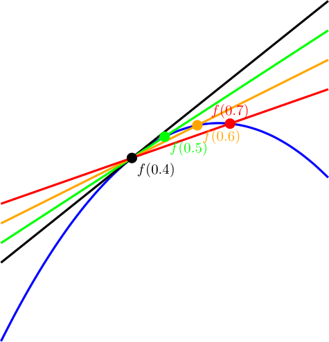
Let’s say that was 2 because we had 3 data pairs. Our three basis functions would be:

Which means that our final Lagrange interpolation function would be:

That is quite a mouth full, but hopefully you understand how we came up with that!
 is just controlPoints[i].x and
  is just controlPoints[i].y.
Math Intuition
The intuition here is that we need to come up with a set of functions to multiply each control point by, such that when the function’s x value is at the control point’s x value, the function should evaluate to 1. When the function’s x value is at a different control points x value, the function should evaluate to 0. The rest of the time, the function can evaluate to whatever it wants, although again, having it have smooth values is nice to making a good curve.
So the first problem is, how do we make a function evaluate to 0 when x is at a different control point?
The easy way would be to multiply a bunch of terms together of this form  , but make sure and not include the x of the actual control point that we are multiplying against.
That is exactly what it does with the numerator in the product notation of the basis function.
Note that is the index of the current control point that we are calculating the basis function for. All values of x, that isn’t the x value of a control point will evaluate to non zero.
The denominator value is there so that when x is the value of the control point that we care about, that the function will evaluate to 1.
It does this by figuring out what the value of the numerator will be when x is at the control point, and then makes that be the value that it divides by, so that it’s 1 at that x value.
Not too much to it. Pretty simple stuff, but powerful as well!
Extending to 2D and Beyond
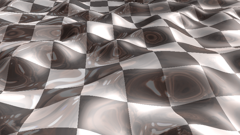
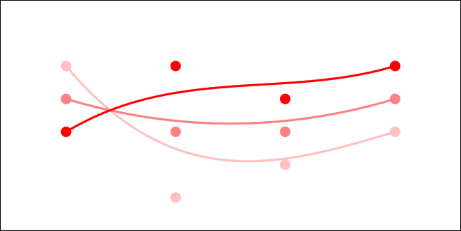
Lagrange interpolation is a one dimensional interpolation scheme, meaning that if you have data points of the form (x,y), it can give you an interpolated y value based on an x value you give it. The interpolation it does can never give two different y values for the same x.
If you want to extend this technique to interpolating a curve through two dimensional data points, or even higher, you need to do interpolation independently for each axis and use a “parametric” value for that axis.
For instance, if you needed to interpolate a curve through 3 dimensional points, you would have data points like this:
X Points = 
Y Points = 
Z Points = 
And then you would interpolate on each axis by the t value to get your X, Y and Z axis values. This should look familiar, because this is how higher dimensional Bezier curves work; you evaluate them per axis based on a parametric value per axis (s,t,u,etc).
You could use the same t values on each axis, or they could be completely independent. You don’t even need to have the same number of points for each axis!
You might wonder how this differs from the standard interpolation in the 2D case. Check the demos in the link section below to really get a grasp of the difference, but in essence, with standard (1D) interpolation, you can never have two x values that evaluate to 2 different y values. Extending it like the above into two dimensions by parameterizing each axis lets you get around that limitation and you can make true 2d shapes.
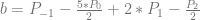
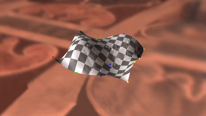
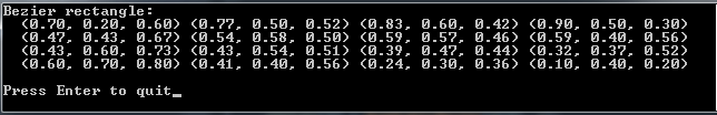
Lastly, it is possible to make Lagrange interpolated surfaces! I won’t go into the details (perhaps a future post!), but if you know how to make a bezier rectangle by doing a tensor product (basically having X axis Bezier curves, multiplied by Y axis Bezier curves), you can accomplish a Lagrange surface in a really similar way.
Sample Code
This sample code is written for readability, but could easily be optimized for faster execution. Also, from what I hear, the second form of Barycentric Lagrange Interpolation is touted as the fastest form of Lagrange interpolation, since many values can be pre-calculated and re-used for different values of x.
#include <stdio.h>
#include <vector>

struct SPoint
{
    float x;
    float y;
};

typedef std::vector<SPoint> TPointList;

void WaitForEnter ()
{
    printf("Press Enter to quit");
    fflush(stdin);
    getchar();
}

// calculates the lagrange basis function y value for control point "controlPointIndex" at x value "x"
float LagrangeBasis (const TPointList& pointList, size_t controlPointIndex, float x)
{
    // this is the pi "inner loop" multiplication work
    float value = 1.0f;
    for (size_t i = 0, c = pointList.size(); i < c; ++i) {
        if (i != controlPointIndex)
            value *= (x - pointList[i].x) / (pointList[controlPointIndex].x - pointList[i].x);
    }
    return value;
}

// returns a value at x, using lagrange interpolation over the specified list of (x,y) pairs
float LagrangeInterpolate (const TPointList& pointList, float x)
{
    // this is the sigma "outer loop" summation work
    float sum = 0.0f;
    for (size_t controlPointIndex = 0, c = pointList.size(); controlPointIndex < c; ++controlPointIndex)
        sum += pointList[controlPointIndex].y * LagrangeBasis(pointList, controlPointIndex, x);
    return sum;
}

int main (int argc, char **argv)
{
    // show some 1d interpolated values
    // note that the points don't need to be sorted on X, but it makes for easier to read examples
    {
        // (x,y) pairs
        const TPointList points =
        {
            { 0.0f, 1.1f },
            { 1.6f, 8.3f },
            { 2.3f, 6.5f },
            { 3.5f, 4.7f },
            { 4.3f, 3.1f },
            { 5.9f, 7.5f },
            { 6.8f, 0.0f }
        };

        // show values interpolated from x = 0, to x = max x
        printf("1d interpolated values.  y = L(t)n");
        const float c_numPoints = 10;
        for (int i = 0; i < c_numPoints; ++i)
        {
            float percent = ((float)i) / (float(c_numPoints - 1));
            float x = points.back().x * percent;
            float y = LagrangeInterpolate(points, x);
            printf("  (%0.2f, %0.2f)n", x, y);
        }
        printf("n");
    }

    // show some 2d interpolated values
    // also note that x and y don't have to have matching t values!
    {
        // (t, x) pairs
        const TPointList pointsX =
        {
            { 0.0, 0.0f},
            { 1.0, 1.6f},
            { 2.0, 2.3f},
            { 3.0, 3.5f},
            { 4.0, 4.3f},
            { 5.0, 5.9f},
            { 6.0, 6.8f}

        };
        // (t, y) pairs
        const TPointList pointsY =
        {
            { 0.0f, 1.1f },
            { 1.0f, 8.3f },
            { 2.0f, 6.5f },
            { 3.0f, 4.7f },
            { 4.0f, 3.1f },
            { 5.0f, 7.5f },
            { 6.0f, 0.0f }
        };

        // show values interpolated from t = 0, to t = max t, on each axis
        printf("2d interpolated values.  x = L(t_x), y = L(t_y)n");
        const float c_numPoints = 10;
        for (int i = 0; i < c_numPoints; ++i)
        {
            float percent = ((float)i) / (float(c_numPoints - 1));

            // calculate x
            float tx = pointsX.back().x * percent;
            float x = LagrangeInterpolate(pointsX, tx);

            // calculate y
            float ty = pointsY.back().x * percent;
            float y = LagrangeInterpolate(pointsY, ty);

            printf("  (%0.2f, %0.2f)n", x, y);
        }
        printf("n");
    }

    WaitForEnter();
    return 0;
}
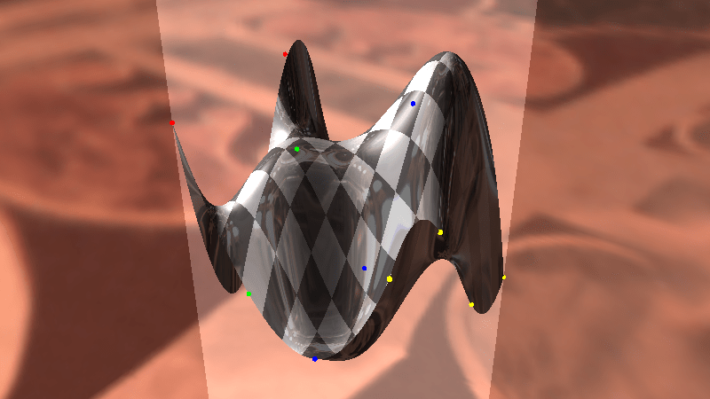
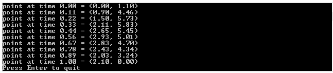
And here’s the programs output:

Final Notes
Now that you know how to do all this stuff I wanted to share a couple more pieces of info.
Firstly, it’s kind of weird to call this “Lagrange Interpolation”. A better term is to call this the “Lagrange Form of Polynomial Interpolation”. The reason for that is that if you have some number of data points, there exists only one unique minimal order polynomial (lowest degree of x possible) that fits those points. That is due to the “unisolvence theorem” that you can read more about here: Wikipedia: Polynomial interpolation.
What that means is that if you were to use a different type of polynomial interpolation – such as newton interpolation – the result you get out is algebraically equivalent to the one you’d get from this Lagrange form. There are pros and cons to using different forms of polynomials, but that’s out of the scope of this post so go read about them if you are interested!
Speaking of that, even though this sample code is focused on interpolation using the Lagrange form, this technique is really great at being able to just come up with some simpler f(x) function that passes through specific data points. In this way, you can kind of “bake out” a custom f(x) function to do interpolation for specific values, that doesn’t need all the moving parts of the Lagrange form. For example, if you make the formula for lagrange interpolation of 3 specific value pairs and then simplify, will get out a simple quadratic function in the form of  !
!
Links
Here are some interactive demos I made to let you play with Lagrange interpolation to get a feel for how it works, and it’s strengths and weaknesses:
One Dimensional Lagrange Interpolation
Two Dimensional Lagrange Interpolation
I also found these links really helpful in finally understanding this topic:
Lagrange Interpolation
Lagrange’s Interpolation Formula
Want to follow the rabbit hole a little deeper? Check out how sinc interpolation relates to the Lagrange form!
The ryg blog: sinc and Polynomial interpolation


 continuity everywhere!
 . The curve at time 0 will be at point
  and the slope will be the same slope as a line would have if going from
  to
to  . The curve at time 1 will be at point
  .
.


 are used to be able to make this interpolation
 and
and  . You subtract the first one from the second and divide by 2*e to get an approximated slope of the function at the specific value of x.

 , subtracts the 1st one from the second one and divides the result by e.


 is the point on the surface that you get after you plug in the parameters.
  and
and  are the parameters to the surface and should be within the range 0 to 1. These are the same thing as the
  you see in Bezier curves, but there are two of them since there are two axes.
 go from 0 to
  and the other makes
  and
and  . The number of control on one axis are multiplied by the number of control points on the other axis.
 and
and  at time
  .
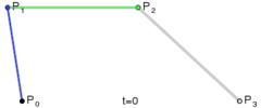
. . A quadratic curve is just a linear interpolation between two curves of degree 1 (aka linear curves). Specifically, you take a linear interpolation between
  , and a linear interpolation between
  , and then take a linear interpolation between those two results. That will give you your quadratic curve.
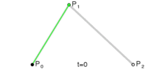
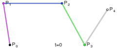
 . A cubic curve is just a linear interpolation between two quadratic curves. Specifically, the first quadratic curve is defined by control points
  .
.
 . A quartic curve is just a linear interpolation between two cubic curves. The first cubic curve is defined by control points
  .
.

 is just
  )
)

 and
and  , using the alpha of the pixel you are writing to determine the weighting for the lerp.
 is already multipled by
  which results in slightly less math:


 are the weightings associated with those control points.
 .
. or
or  or
or  .
. , instead of
  , we come up with the equation in the next section.