One way to look at sounds is to think about what frequencies they contain, at which strengths (amplitudes), and how those amplitudes change over time.
For instance, if you remember the details of the post about how to synthesis a drum sound (DIY Synth: Basic Drum), a drum has low frequencies, but also, the frequencies involved get lower over the duration, which gives it that distinctive sound.
Being able to analyze the frequency components of a sound you want to mimic, and then being able to generate audio samples based on a description of frequency components over time is a powerful tool in audio synthesis.
This post will talk about exactly that, using both oscillators as well as the inverse fast Fourier transform (IFFT).
We’ve already gone over the basics of using oscillators to create sounds in a previous post so we’ll start with IFFT. For a refresher on those basics of additive synthesis check out this link: DIY Synth 3: Sampling, Mixing, and Band Limited Wave Forms
All sample sound files were generated with the sample code at the end of this post. The sample code is a single, standalone c++ file which only includes standard headers and doesn’t rely on any libraries. You should be able to compile it and start using the techniques from this post right away!
What is the IFFT?
Audio samples are considered samples in the “time domain”. If you instead describe sound based on what frequencies they contain, what amplitudes they are at, and what phase (angle offset) the sinusoid wave starts at, what you have is samples in the “frequency domain”.
The process for converting time domain to frequency domain is called the “Fourier Transform”. If you want to go the opposite way, and convert frequency domain into time domain, you use the “Inverse Fourier Transform”.
These transforms come in two flavors: continuous and discrete.
The continuous Fourier transform and continuous inverse Fourier transform work with continuous functions. That is, they will transform a function from time domain to frequency domain, or from frequency domain to time domain.
The discrete version of the fourier transform – often refered to as DFT, short for “discrete fourier transform” – and inverse fourier transform work with data samples instead of functions.
Naively computing the DFT or IDFT is a very processor intensive operation. Luckily for us, there is an algorithm called “Fast Fourier Transform” or FFT that can do it a lot faster, if you are ok with the constraints of the data it gives you. It also has an inverse, IFFT.
IFFT is what we are going to be focusing on in this post, to convert frequency domain samples into time domain samples. Also, like i said above, we are also going to be using oscillators to achieve the same result!
Using the IFFT
Here’s something interesting… where time domain samples are made up of “real numbers” (like 0.5 or -0.9 or even 1.5 etc), frequency domain samples are made up of complex numbers, which are made up of a real number and an imaginary number. An example of a complex number is “3.1 + 2i” where i is the square root of negative 1.
If you look at the complex number as a 2d vector, the magnitude of the vector is the amplitude of the frequency, and the angle of the vector is the phase (angle) that the sinusoid (cosine wave) starts at for that frequency component.
You can use these formulas to create the complex number values:
real = amplitude * cos(phase);
imaginary = amplitude * sin(phase);
Or you could use std::polar if you want to (:
BTW thinking of complex numbers as 2d vectors might be a little weird but there’s precedent. Check this out: Using Imaginary Numbers To Rotate 2D Vectors
When using the IFFT, the number of frequency domain samples you decide to use is what decides the frequencies of those samples. After preforming the IFFT, you will also have the same number of time domain samples as frequency domain samples you started with. That might sound like it’s going to be complex, but don’t worry, it’s actually pretty simple!
Let’s say that you have 4 buckets of frequency domain data, that means you will end up with 4 time domain audio samples after running IFFT. Here are the frequencies that each frequency domain sample equates to:
- index 0: 0hz. This is the data for the 0hz frequency, or DC… yes, as in DC current! DC represents a constant added to all samples in the time domain. If you put a value in only this bucket and run the IFFT, all samples will be the same constant value.
- index 1: 1hz. If you put a value in only this bucket and run the IFFT, you’ll end up with one full cosine wave (0-360 degrees aka 0-2pi radians), across the 4 time domain samples. 4 samples isn’t very many samples for a cosine wave though so it will look pretty blocky, but those 4 samples will be correct!
- index 2: 2hz. If you put a value in only this bucket and run the IFFT, you’ll end up with two full cosine waves (0-720 degrees aka 0-4pi radians) across the 4 time domain samples.
- index 3: -1hz.
You might wonder what that negative frequency at index 3 is all about. A negative frequency probably seems weird, but it’s really the same as it’s positive frequency, just with a negative phase. It’s basically a cosine wave that decreases in angle as it goes, instead of increasing.
Why is it there though? Well, there’s something called the Nyquist–Shannon Sampling Theorem which states that if you have N time domain audio samples, the maximum frequency you can store in those audio samples is N/2 cycles. That frequency is called the Nyquist frequency and any frequency above that results in “aliasing”. If you’ve ever seen a car tire spin in reverse on tv when the care was moving forward, that is an example of the same aliasing I’m talking about. In manifests in audio as high pitches and in general terrible sounding sound. Before I knew how to avoid aliasing in audio, my now wife used to complain that my sounds hurt her ears. Once i removed the aliasing, she says it no longer hurts her ears. Go back and check the early DIY synth posts for audible examples of aliasing (;
Since we have 4 frequency domain samples, which translates to 4 time domain audio samples, we can only store up to 2hz, and anything above that will alias and seem to go backwards. That’s why index 3 is -1hz instead of 3hz.
So basically, if you have N frequency domain samples (or bins as they are sometimes called), the first bin, at index 0, is always 0hz / DC. Then from 1 up to N/2, the frequency of the bin is equal to it’s index. Then, at N/2+1 up to N-1, there are negative frequencies (frequencies beyond the Nyquist frequency) reflected in that upper half of the bins, starting at N/2 and counting back up to -1.
In many common situations (including the ones we are facing in this post), you don’t need to worry about the negative frequency bins. You can leave them as zero if doing IFFT work, or ignore their values if doing FFT then IFFT work.
Ready for one last piece of complexity? I hope so… it’s the last before moving onto the next step! 😛
Sounds are obviously much longer than 4 samples, so a 4 bin (sample) IFFT just isn’t going to cut it. 1000 bins would to be too few, and Frankly, at 44,100 samples per second (a common audio sampling rate), 88,200 bins is only 2 seconds of audio which isn’t very much at all! Even with the “Fast Fourier Transform” (FFT), that is a huge number of bins and would take a long time to calculate.
One way to deal with this would be to have fewer bins than audio samples that you want to end up with, use IFFT to generate the audio samples, and then use interpolation to get the audio samples between the ones generated by IFFT. We aren’t going to be doing that today but if you like the option, you can most certainly use it!
One of the ways we are going to deal with using a small number of bins to generate a lot of noise is that we are going to use the IFFT to generate wave forms, and then we are going to repeat those wave forms several times.
Another one of the things we are going to do is use IFFT bins to generate a small number of samples, and then modify the IFFT bins to generate the next number of samples, repeating until we have all of our audio samples generated.
In both cases, the frequency buckets need some conversion from the IFFT bin frequencies to the frequencies as they will actually appear in the final audio samples.
To calculate the true frequency of an FFT bin, you can use this formula:
frequency = binNumber * sampleRate / numBins;
Where binNumber is the IFFT bin number, sampleRate is how many samples the resulting sound has per second, and numBins is the total number of IFFT bins.
Simple Wave Forms
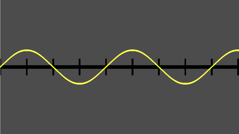
The simplest of the wave forms you can create is a cosine wave. You just put the complex number “1 + 0i” into one of the IFFT bins, that represents an amplitude of 1.0 and a starting phase of 0 degrees. After you do that and run ifft, you’ll get a nice looking cosine wave:
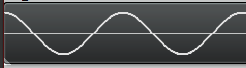
Note that the wave repeats multiple times. This is because I repeat the IFFT data over and over. If I didn’t repeat the IFFT data, the number of cycles that would appear would depend completely on which IFFT bin I used. If I used bin 1, it would have only one cycle. If i used bin 2, it would have two cycles.
Also note that since the IFFT deals with INTEGER frequencies only, that means that the wave forms begin and end at the same phase (angle) and thus the same amplitude, which means that if you repeat them end to end, there will be no discontinuities or popping. Pretty cool huh?
If you instead put in the complex number “0 – 1i” into one of the IFFT bins, that represents an amplitude of 1.0 and a starting phase of 270 degrees (or -90 degrees), which results in a sine wave:
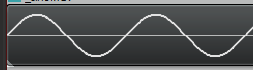
We don’t have to stop there though. Once again thinking back to the info in DIY Synth 3: Sampling, Mixing, and Band Limited Wave Forms, the frequency components of a saw wave are described as:
If you have a saw wave of frequency 100, that means it contains a sine wave of frequency 100 (1 * fundamental frequency), another of frequency 200 (2 * fundamental frequency), another of 300 (3 * fundamental frequency) and so on into infinity.
The amplitude (volume) of each sine wave (harmonic) is 1 over the harmonic number. So in our example, the sine wave at frequency 100 has an amplitude of 1 (1/1). The sine wave at frequency 200 has an amplitude of 0.5 (1/2), the sine wave at frequency 300 has an amplitude of 0.333 (1/3) and so on into infinity.
After that you’ll need to multiply your sample by 2 / PI to get back to a normalized amplitude.
We can describe the same thing in IFFT frequency bins believe it or not!
Let’s say that we have 50 bins and that we want a 5hz saw wave. The first harmonic is 5hz and should be full amplitude, so we put an entry in bin 5 for amplitude 1.0 * 2/pi and phase -90 degrees (to make a sine wave instead of a cosine wave).
The next harmonic should be double the frequency, and 1/2 the amplitude, so in bin 10 (double the frequency of bin 5), we put an entry for amplitude 0.5 * 2/pi, phase -90 degrees. Next should be triple the original frequency at 1/3 the amplitude, so at bin 15 we put amplitude 0.33 * 2/pi, phase -90 degrees. Then, bin 20 gets amplitude 0.25 * 2/pi, -90 degrees phase. Bin 25 is the Nyquist frequency so we should stop here, and leave the actual Nyquist frequency empty.
If you run the IFFT on that, you’ll get a bandlimited saw wave!
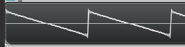
You can do the same for bandlimited triangle and square waves, and also you can use a random phase and amplitude for each bin to generate noise! The source code for this post generates those in fact (:
Phase Adjusted Wave Forms
While we are dealing in frequency space, I want to run something kind of gnarly by you. Using the technique described above, you can add frequencies with specific amplitudes to make a band limited saw wave. But, believe it or not, the starting phase of the frequencies don’t have to be -90 degrees. If you use a different phase, you’ll get a resulting wave form that looks different but sounds the same. Check these out, it’s a trip!
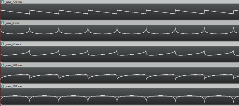
Here are the sound files pictured above, so you can hear that they really do all sound the same!
270 degrees
0 degrees
60 degrees
120 degrees
180 degrees
Bins Changing Over Time
If you are like me, when you think about designing sound in the frequency domain you think everything must be rainbows and glitter, and that you have no limitations and everything is wonderful.
Well, as happens so many times when the rubber hits the road, that isn’t quite true. Let’s go through an example of using IFFT on some bins that change over time so I can show you a really big limitation with IFFT.
In our example, let’s say that we have a single frequency in our IFFT data (so we are generating a single sinusoid wave) but that we want it’s amplitude (volume) to change over time. Let’s say we want the amplitude of the wave to be controlled by another sinusoid, so that it smoothly goes up and down in amplitude over time.
We immediately hit two problems, but the first is more obvious if you listen:
IFFTTest1.wav
Hear all that popping? It’s basically making a discontinuity at every IFFT window because we are changing the amplitude at the edge of each window. We can’t change it during the window (caveat: without some pretty advanced math i won’t go into), so changing at the end of the window is our only option. Check out this image to see the problem visually:

We can fix those discontinuities. If we change the phase of the wave from cosine (0 degrees) to sine (270 degrees), we make it so that the edge of the window is always at amplitude 0 (sine(0) = 0, while cos(0) = 1!). This means that when we change the amplitude of the wave, since it happens when the wave is at zero, there is no discontinuity, and so no more pops:

Let’s have a listen:
IFFTTest2.wav
WHAT?! There is still some periodic noise… it is tamed a little bit but not fixed. The reason for this is that even though we are first order continuous we aren’t 2nd order continuous (etc). So, by having a jump in amplitude, even constraining it at zero crossings, we’ve essentially added some frequencies into our resulting sound wave that we didn’t want to add, which we can hear in the results.
So yeah… basically, if you want to change your IFFT bins over time, you are going to have some audio artifacts from doing that. Boo hoo!
There are ways around this. One way involves complex math to add frequencies to your bins that make it APPEAR as if you are adjusting the amplitude of the wave smoothly over the duration of the window. Another way involves doing things like overlapping the output of your IFFT windows and blending between them. There are other ways too, including some IDFT algorithms which do allow you to alter the amplitude over time in a window, but are costlier to compute.
Anyways, you can also just generate the sound descibed in your IFFT bins with oscillators, literally adding together all the frequencies with the specified phase offsets to make the correct resulting time domain samples. I’ve done just that to solve the popping problem as well as the issue where you can’t have smooth volume adjustments because you can only change amplitude at the end of each window:
IFFTTest3.wav
You can also see it in action:

Here’s another failure case to check out:

drums_ifft.wav – made with ifft
drums_osc.wav – made with oscillators
Convolution
If you read the post about convolution reverb (DIY Synth: Convolution Reverb & 1D Discrete Convolution of Audio Samples), you’ll recall that convolution is super slow, but that convolution in the time domain is equivelant to multiplication in the frequency domain.
We are in the frequency domain, so how about we try some convolution?!
Let’s multiply the bins of a 1hz saw wave and a 1hz square wave and see what we get if we IFFT the result:
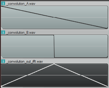
That result is definitely not right. First of all, the convolution is the same length as the inputs, when it should be length(a)+length(b)-1 samples. Basically it should be twice as long as it is.
Secondly, that is not what the convolution looks like. Doing convolution in the time domain of those samples looks like this:

So what’s the deal? Well as it turns out, when you do multiplication in the frequency domain, you are really doing CIRCULAR convolution, which is a bit different than the convolution i described before which is LINEAR convolution. Circular convolution is essentially used for cyclical data (or functions) and basically makes it so that if you try to read “out of bounds”, it will wrap around and use an in bounds value instead. It’s kind of like “texture wrap” if you are a graphics person.
Normally how this is gotten around, when doing convolution in the frequency domain, is to put a bunch of zeros on the end of your time domain samples before you bring them into the frequency domain. You pad them with those zeros to be the correct size (length(a)+length(b)-1, or longer is fine too) and then when you end up doing the “circular convolution”, there are no “out of bounds” values looked at, and you end up with the linear convolution output, even though you technically did circular convolution.
Unfortunately, since we are STARTING in frequency domain and have no time domain samples to bad before going into frequency domain, we are basically out of luck. I’ve tried asking DSP experts and nobody I talked to knows of a way to start in frequency domain and zero pad the time domain so that you could do a linear convolution – at least nobody knows of GENERAL case solution.
Those same experts though say that circular convolution isn’t a bad thing, and is many times exactly what you want to do, or is a fine stand in for linear convolution. I’m sure we’ll explore that in a future post (:
In the example code, i also have the code generate the circular convolution in the time domain so that you can confirm that circular convolution is really what is going on in the above image, when working in frequency domain.
Strike Two IFFT!
Luckily using IDFT to generate sounds (sometimes called Fourier Synthesis) isn’t across the board a losing strategy. If you want a static, repeating wave form, it can be really nice. Or, for dynamic waave forms, if you change your amplitude only a very small amount across window samples, it won’t noticeably degrade the quality of your audio.
The neat thing about IFFT is that it’s a “constant time process”. When using oscillators, the more frequencies you want to appear, the more computationally expensive it gets. With IFFT, it doesn’t matter if all the bins are full or empty or somewhere inbetween, it has the same computational complexity.
Here’s a non trivial sound generated both with IFFT and Oscillators. The difference is pretty negligible right?
alien_ifft.wav – made with IFFT
alien_osci.wav – made with oscillators
Sample Code
#define _CRT_SECURE_NO_WARNINGS

#include
#include
#include
#include
#include
#include
#include
#include
#include
#include
#include
#include

#define _USE_MATH_DEFINES
#include

//=====================================================================================
// SNumeric - uses phantom types to enforce type safety
//=====================================================================================
template
struct SNumeric
{
public:
    explicit SNumeric(const T &value) : m_value(value) { }
    SNumeric() : m_value() { }
    inline T& Value() { return m_value; }
    inline const T& Value() const { return m_value; }

    typedef SNumeric TType;
    typedef T TInnerType;

    // Math Operations
    TType operator+ (const TType &b) const
    {
        return TType(this->Value() + b.Value());
    }

    TType operator- (const TType &b) const
    {
        return TType(this->Value() - b.Value());
    }

    TType operator* (const TType &b) const
    {
        return TType(this->Value() * b.Value());
    }

    TType operator/ (const TType &b) const
    {
        return TType(this->Value() / b.Value());
    }

    TType operator% (const TType &b) const
    {
        return TType(this->Value() % b.Value());
    }

    TType& operator+= (const TType &b)
    {
        Value() += b.Value();
        return *this;
    }

    TType& operator-= (const TType &b)
    {
        Value() -= b.Value();
        return *this;
    }

    TType& operator*= (const TType &b)
    {
        Value() *= b.Value();
        return *this;
    }

    TType& operator/= (const TType &b)
    {
        Value() /= b.Value();
        return *this;
    }

    TType& operator++ ()
    {
        Value()++;
        return *this;
    }

    TType& operator-- ()
    {
        Value()--;
        return *this;
    }

    // Extended Math Operations
    template
    T Divide(const TType &b)
    {
        return ((T)this->Value()) / ((T)b.Value());
    }

    // Logic Operations
    bool operatorValue() < b.Value();
    }
    bool operatorValue()  (const TType &b) const {
        return this->Value() > b.Value();
    }
    bool operator>= (const TType &b) const {
        return this->Value() >= b.Value();
    }
    bool operator== (const TType &b) const {
        return this->Value() == b.Value();
    }
    bool operator!= (const TType &b) const {
        return this->Value() != b.Value();
    }

private:
    T m_value;
};

//=====================================================================================
// Typedefs
//=====================================================================================

typedef uint8_t uint8;
typedef uint16_t uint16;
typedef uint32_t uint32;
typedef int16_t int16;
typedef int32_t int32;

// type safe types!
typedef SNumeric        TFrequency;
typedef SNumeric           TFFTBin;
typedef SNumeric          TTimeMs;
typedef SNumeric            TTimeS;
typedef SNumeric         TSamples;
typedef SNumeric     TFractionalSamples;
typedef SNumeric         TDecibels;
typedef SNumeric        TAmplitude;
typedef SNumeric          TRadians;
typedef SNumeric          TDegrees;

//=====================================================================================
// Constants
//=====================================================================================

static const float c_pi = (float)M_PI;
static const float c_twoPi = c_pi * 2.0f;

//=====================================================================================
// Structs
//=====================================================================================

struct SSoundSettings
{
    TSamples        m_sampleRate;
    TSamples        m_sampleCount;
};

//=====================================================================================
// Conversion Functions
//=====================================================================================

inline TFFTBin FrequencyToFFTBin(TFrequency frequency, TFFTBin numBins, TSamples sampleRate)
{
    // bin = frequency * numBin / sampleRate
    return TFFTBin((uint32)(frequency.Value() * (float)numBins.Value() / (float)sampleRate.Value()));
}

inline TFrequency FFTBinToFrequency(TFFTBin bin, TFFTBin numBins, TSamples sampleRate)
{
    // frequency = bin * SampleRate / numBins
    return TFrequency((float)bin.Value() * (float)sampleRate.Value() / (float)numBins.Value());
}

inline TRadians DegreesToRadians(TDegrees degrees)
{
    return TRadians(degrees.Value() * c_pi / 180.0f);
}

inline TDegrees RadiansToDegrees(TRadians radians)
{
    return TDegrees(radians.Value() * 180.0f / c_pi);
}

inline TDecibels AmplitudeToDB(TAmplitude volume)
{
    return TDecibels(20.0f * log10(volume.Value()));
}

inline TAmplitude DBToAmplitude(TDecibels dB)
{
    return TAmplitude(pow(10.0f, dB.Value() / 20.0f));
}

TTimeS SamplesToSeconds(const SSoundSettings &s, TSamples samples)
{
    return TTimeS(samples.Divide(s.m_sampleRate));
}

TSamples SecondsToSamples(const SSoundSettings &s, TTimeS seconds)
{
    return TSamples((int)(seconds.Value() * (float)s.m_sampleRate.Value()));
}

TSamples MilliSecondsToSamples(const SSoundSettings &s, TTimeMs milliseconds)
{
    return SecondsToSamples(s, TTimeS((float)milliseconds.Value() / 1000.0f));
}

TTimeMs SecondsToMilliseconds(TTimeS seconds)
{
    return TTimeMs((uint32)(seconds.Value() * 1000.0f));
}

TFrequency Frequency(float octave, float note)
{
    /* frequency = 440×(2^(n/12))
    Notes:
    0  = A
    1  = A#
    2  = B
    3  = C
    4  = C#
    5  = D
    6  = D#
    7  = E
    8  = F
    9  = F#
    10 = G
    11 = G# */
    return TFrequency((float)(440 * pow(2.0, ((double)((octave - 4) * 12 + note)) / 12.0)));
}

template
T AmplitudeToAudioSample(const TAmplitude& in)
{
    const T c_min = std::numeric_limits::min();
    const T c_max = std::numeric_limits::max();
    const float c_minFloat = (float)c_min;
    const float c_maxFloat = (float)c_max;

    float ret = in.Value() * c_maxFloat;

    if (ret  c_maxFloat)
        return c_max;

    return (T)ret;
}

//=====================================================================================
// Audio Utils
//=====================================================================================

void EnvelopeSamples(std::vector& samples, TSamples envelopeTimeFrontBack)
{
    const TSamples c_frontEnvelopeEnd(envelopeTimeFrontBack);
    const TSamples c_backEnvelopeStart(samples.size() - envelopeTimeFrontBack.Value());

    for (TSamples index(0), numSamples(samples.size()); index < numSamples; ++index)
    {
        // calculate envelope
        TAmplitude envelope(1.0f);
        if (index < c_frontEnvelopeEnd)
            envelope = TAmplitude(index.Divide(envelopeTimeFrontBack));
        else if (index > c_backEnvelopeStart)
            envelope = TAmplitude(1.0f) - TAmplitude((index - c_backEnvelopeStart).Divide(envelopeTimeFrontBack));

        // apply envelope
        samples[index.Value()] *= envelope;
    }
}

void NormalizeSamples(std::vector& samples, TAmplitude maxAmplitude)
{
    // nothing to do if no samples
    if (samples.size() == 0)
        return;

    // 1) find the largest absolute value in the samples.
    TAmplitude largestAbsVal = TAmplitude(abs(samples.front().Value()));
    std::for_each(samples.begin() + 1, samples.end(), [&largestAbsVal](const TAmplitude &a)
        {
            TAmplitude absVal = TAmplitude(abs(a.Value()));
            if (absVal > largestAbsVal)
                largestAbsVal = absVal;
        }
    );

    // 2) adjust largestAbsVal so that when we divide all samples, none will be bigger than maxAmplitude
    // if the value we are going to divide by is <= 0, bail out
    largestAbsVal /= maxAmplitude;
    if (largestAbsVal <= TAmplitude(0.0f))
        return;

    // 3) divide all numbers by the largest absolute value seen so all samples are [-maxAmplitude,+maxAmplitude]
    for (TSamples index(0), numSamples(samples.size()); index < numSamples; ++index)
        samples[index.Value()] = samples[index.Value()] / largestAbsVal;
}

//=====================================================================================
// Wave File Writing Code
//=====================================================================================
struct SMinimalWaveFileHeader
{
    //the main chunk
    unsigned char m_szChunkID[4];      //0
    uint32        m_nChunkSize;        //4
    unsigned char m_szFormat[4];       //8

    //sub chunk 1 "fmt "
    unsigned char m_szSubChunk1ID[4];  //12
    uint32        m_nSubChunk1Size;    //16
    uint16        m_nAudioFormat;      //18
    uint16        m_nNumChannels;      //20
    uint32        m_nSampleRate;       //24
    uint32        m_nByteRate;         //28
    uint16        m_nBlockAlign;       //30
    uint16        m_nBitsPerSample;    //32

    //sub chunk 2 "data"
    unsigned char m_szSubChunk2ID[4];  //36
    uint32        m_nSubChunk2Size;    //40

    //then comes the data!
};

//this writes a wave file
template
bool WriteWaveFile(const char *fileName, const std::vector &samples, const SSoundSettings &sound)
{
    //open the file if we can
    FILE *file = fopen(fileName, "w+b");
    if (!file)
        return false;

    //calculate bits per sample and the data size
    const int32 bitsPerSample = sizeof(T) * 8;
    const int dataSize = samples.size() * sizeof(T);

    SMinimalWaveFileHeader waveHeader;

    //fill out the main chunk
    memcpy(waveHeader.m_szChunkID, "RIFF", 4);
    waveHeader.m_nChunkSize = dataSize + 36;
    memcpy(waveHeader.m_szFormat, "WAVE", 4);

    //fill out sub chunk 1 "fmt "
    memcpy(waveHeader.m_szSubChunk1ID, "fmt ", 4);
    waveHeader.m_nSubChunk1Size = 16;
    waveHeader.m_nAudioFormat = 1;
    waveHeader.m_nNumChannels = 1;
    waveHeader.m_nSampleRate = sound.m_sampleRate.Value();
    waveHeader.m_nByteRate = sound.m_sampleRate.Value() * 1 * bitsPerSample / 8;
    waveHeader.m_nBlockAlign = 1 * bitsPerSample / 8;
    waveHeader.m_nBitsPerSample = bitsPerSample;

    //fill out sub chunk 2 "data"
    memcpy(waveHeader.m_szSubChunk2ID, "data", 4);
    waveHeader.m_nSubChunk2Size = dataSize;

    //write the header
    fwrite(&waveHeader, sizeof(SMinimalWaveFileHeader), 1, file);

    //write the wave data itself, converting it from float to the type specified
    std::vector outSamples;
    outSamples.resize(samples.size());
    for (size_t index = 0; index < samples.size(); ++index)
        outSamples[index] = AmplitudeToAudioSample(samples[index]);
    fwrite(&outSamples[0], dataSize, 1, file);

    //close the file and return success
    fclose(file);
    return true;
}

//=====================================================================================
// FFT / IFFT
//=====================================================================================

// Thanks RosettaCode.org!
// http://rosettacode.org/wiki/Fast_Fourier_transform#C.2B.2B
// In production you'd probably want a non recursive algorithm, but this works fine for us

// for use with FFT and IFFT
typedef std::complex Complex;
typedef std::valarray CArray;

// Cooley–Tukey FFT (in-place)
void fft(CArray& x)
{
    const size_t N = x.size();
    if (N <= 1) return;

    // divide
    CArray even = x[std::slice(0, N/2, 2)];
    CArray  odd = x[std::slice(1, N/2, 2)];

    // conquer
    fft(even);
    fft(odd);

    // combine
    for (size_t k = 0; k < N/2; ++k)
    {
        Complex t = std::polar(1.0f, -2 * c_pi * k / N) * odd[k];
        x[k    ] = even[k] + t;
        x[k+N/2] = even[k] - t;
    }
}

// inverse fft (in-place)
void ifft(CArray& x)
{
    // conjugate the complex numbers
    x = x.apply(std::conj);

    // forward fft
    fft( x );

    // conjugate the complex numbers again
    x = x.apply(std::conj);

    // scale the numbers
    x /= (float)x.size();
}

//=====================================================================================
// Wave forms
//=====================================================================================

void SineWave(CArray &frequencies, TFFTBin bin, TRadians startingPhase)
{
    // set up the single harmonic
    frequencies[bin.Value()] = std::polar(1.0f, startingPhase.Value());
}

void SawWave(CArray &frequencies, TFFTBin bin, TRadians startingPhase)
{
    // set up each harmonic
    const float volumeAdjustment = 2.0f / c_pi;
    const size_t bucketWalk = bin.Value();
    for (size_t harmonic = 1, bucket = bin.Value(); bucket < frequencies.size() / 2; ++harmonic, bucket += bucketWalk)
        frequencies[bucket] = std::polar(volumeAdjustment / (float)harmonic, startingPhase.Value());
}

void SquareWave(CArray &frequencies, TFFTBin bin, TRadians startingPhase)
{
    // set up each harmonic
    const float volumeAdjustment = 4.0f / c_pi;
    const size_t bucketWalk = bin.Value() * 2;
    for (size_t harmonic = 1, bucket = bin.Value(); bucket < frequencies.size() / 2; harmonic += 2, bucket += bucketWalk)
        frequencies[bucket] = std::polar(volumeAdjustment / (float)harmonic, startingPhase.Value());
}

void TriangleWave(CArray &frequencies, TFFTBin bin, TRadians startingPhase)
{
    // set up each harmonic
    const float volumeAdjustment = 8.0f / (c_pi*c_pi);
    const size_t bucketWalk = bin.Value() * 2;
    for (size_t harmonic = 1, bucket = bin.Value(); bucket < frequencies.size() / 2; harmonic += 2, bucket += bucketWalk, startingPhase *= TRadians(-1.0f))
        frequencies[bucket] = std::polar(volumeAdjustment / ((float)harmonic*(float)harmonic), startingPhase.Value());
}

void NoiseWave(CArray &frequencies, TFFTBin bin, TRadians startingPhase)
{
    // give a random amplitude and phase to each frequency
    for (size_t bucket = 0; bucket < frequencies.size() / 2; ++bucket)
    {
        float amplitude = static_cast  (rand()) / static_cast  (RAND_MAX);
        float phase = 2.0f * c_pi * static_cast  (rand()) / static_cast  (RAND_MAX);
        frequencies[bucket] = std::polar(amplitude, phase);
    }
}

//=====================================================================================
// Tests
//=====================================================================================

template
void ConsantBins(
    const W &waveForm,
    TFrequency &frequency,
    bool repeat,
    const char *fileName,
    bool normalize,
    TAmplitude multiplier,
    TRadians startingPhase = DegreesToRadians(TDegrees(270.0f))
)
{
    const TFFTBin c_numBins(4096);

    //our desired sound parameters
    SSoundSettings sound;
    sound.m_sampleRate = TSamples(44100);
    sound.m_sampleCount = MilliSecondsToSamples(sound, TTimeMs(500));

    // allocate space for the output file and initialize it
    std::vector samples;
    samples.resize(sound.m_sampleCount.Value());
    std::fill(samples.begin(), samples.end(), TAmplitude(0.0f));

    // make test data
    CArray data(c_numBins.Value());
    waveForm(data, FrequencyToFFTBin(frequency, c_numBins, sound.m_sampleRate), startingPhase);

    // inverse fft - convert from frequency domain (frequencies) to time domain (samples)
    // need to scale up amplitude before fft
    data *= (float)data.size();
    ifft(data);

    // convert to samples
    if (repeat)
    {
        //repeat results in the output buffer
        size_t dataSize = data.size();
        for (size_t i = 0; i < samples.size(); ++i)
            samples[i] = TAmplitude((float)data[i%dataSize].real());
    }
    else
    {
        //put results in the output buffer once.  Useful for debugging / visualization
        for (size_t i = 0; i < samples.size() && i < data.size(); ++i)
            samples[i] = TAmplitude((float)data[i].real());
    }

    // normalize our samples if we should
    if (normalize)
        NormalizeSamples(samples, DBToAmplitude(TDecibels(-3.0f)));

    // apply the multiplier passed in
    std::for_each(samples.begin(), samples.end(), [&](TAmplitude& amplitude) {
        amplitude *= multiplier;
    });

    // write the wave file
    WriteWaveFile(fileName, samples, sound);
}

void Convolve_Circular(const std::vector& a, const std::vector& b, std::vector& result)
{
    // NOTE: Written for readability, not efficiency
    TSamples ASize(a.size());
    TSamples BSize(b.size());

    // NOTE: the circular convolution result doesn't have to be the size of a, i just chose this size to match the ifft
    // circular convolution output.
    result.resize(ASize.Value());
    std::fill(result.begin(), result.end(), TAmplitude(0.0f));

    for (TSamples outputSampleIndex(0), numOutputSamples(ASize); outputSampleIndex < numOutputSamples; ++outputSampleIndex)
    {
        TAmplitude &outputSample = result[outputSampleIndex.Value()];
        for (TSamples sampleIndex(0), numSamples(ASize); sampleIndex < numSamples; ++sampleIndex)
        {
            TSamples BIndex = (outputSampleIndex + ASize - sampleIndex) % ASize;
            if (BIndex < BSize)
            {
                const TAmplitude &ASample = a[sampleIndex.Value()];
                const TAmplitude &BSample = b[BIndex.Value()];
                outputSample += BSample * ASample;
            }
        }
    }
}

void Convolve_Linear(const std::vector& a, const std::vector& b, std::vector& result)
{
    // NOTE: Written for readability, not efficiency
    TSamples ASize(a.size());
    TSamples BSize(b.size());

    result.resize(ASize.Value() + BSize.Value() - 1);
    std::fill(result.begin(), result.end(), TAmplitude(0.0f));

    for (TSamples outputSampleIndex(0), numOutputSamples(result.size()); outputSampleIndex < numOutputSamples; ++outputSampleIndex)
    {
        TAmplitude &outputSample = result[outputSampleIndex.Value()];
        for (TSamples sampleIndex(0), numSamples(ASize); sampleIndex = sampleIndex)
            {
                TSamples BIndex = outputSampleIndex - sampleIndex;
                if (BIndex < BSize)
                {
                    const TAmplitude &ASample = a[sampleIndex.Value()];
                    const TAmplitude &BSample = b[BIndex.Value()];
                    outputSample += BSample * ASample;
                }
            }
        }
    }
}


template
void DoConvolution(const W1 &waveForm1, const W2 &waveForm2)
{
    const TFFTBin c_numBins(4096);

    //our desired sound parameters
    SSoundSettings sound;
    sound.m_sampleRate = TSamples(44100);
    sound.m_sampleCount = TSamples(c_numBins.Value());

    // make the frequency data for wave form 1
    CArray data1(c_numBins.Value());
    waveForm1(data1, TFFTBin(1), DegreesToRadians(TDegrees(270.0f)));

    // make the frequency data for wave form 2
    CArray data2(c_numBins.Value());
    waveForm2(data2, TFFTBin(1), DegreesToRadians(TDegrees(270.0f)));

    // do circular convolution in time domain by doing multiplication in the frequency domain
    CArray data3(c_numBins.Value());
    data3 = data1 * data2;

    // write out the first convolution input (in time domain samples)
    std::vector samples1;
    samples1.resize(sound.m_sampleCount.Value());
    std::fill(samples1.begin(), samples1.end(), TAmplitude(0.0f));
    {
        data1 *= (float)data1.size();
        ifft(data1);

        // convert to samples
        for (size_t i = 0; i < samples1.size() && i < data1.size(); ++i)
            samples1[i] = TAmplitude((float)data1[i].real());

        // write the wave file
        WriteWaveFile("_convolution_A.wav", samples1, sound);
    }

    // write out the second convolution input (in time domain samples)
    std::vector samples2;
    samples2.resize(sound.m_sampleCount.Value());
    std::fill(samples2.begin(), samples2.end(), TAmplitude(0.0f));
    {
        data2 *= (float)data2.size();
        ifft(data2);

        // convert to samples
        for (size_t i = 0; i < samples2.size() && i < data2.size(); ++i)
            samples2[i] = TAmplitude((float)data2[i].real());

        // write the wave file
        WriteWaveFile("_convolution_B.wav", samples2, sound);
    }

    // write the result of the convolution (in time domain samples)
    {
        data3 *= (float)data3.size();
        ifft(data3);

        // convert to samples
        std::vector samples3;
        samples3.resize(sound.m_sampleCount.Value());
        for (size_t i = 0; i < samples3.size() && i < data3.size(); ++i)
            samples3[i] = TAmplitude((float)data3[i].real());

        // write the wave file
        NormalizeSamples(samples3, TAmplitude(1.0f));
        WriteWaveFile("_convolution_out_ifft.wav", samples3, sound);
    }

    // do linear convolution in the time domain and write out the wave file
    {
        std::vector samples4;
        Convolve_Linear(samples1, samples2, samples4);
        NormalizeSamples(samples4, TAmplitude(1.0f));
        WriteWaveFile("_convolution_out_lin.wav", samples4, sound);
    }

    // do circular convolution in time domain and write out the wave file
    {
        std::vector samples4;
        Convolve_Circular(samples1, samples2, samples4);
        NormalizeSamples(samples4, TAmplitude(1.0f));
        WriteWaveFile("_convolution_out_cir.wav", samples4, sound);
    }
}

//=====================================================================================
// Frequency Over Time Track Structs
//=====================================================================================

struct SBinTrack
{
    SBinTrack() { }

    SBinTrack(
        TFFTBin bin,
        std::function amplitudeFunction,
        TRadians phase = DegreesToRadians(TDegrees(270.0f))
    )
        : m_bin(bin)
        , m_amplitudeFunction(amplitudeFunction)
        , m_phase(phase) {}

    TFFTBin                                     m_bin;
    std::function   m_amplitudeFunction;
    TRadians                                    m_phase;
};

//=====================================================================================
// Frequency Amplitude Over Time Test
//=====================================================================================

void TracksToSamples_IFFT_Window(const std::vector &tracks, CArray &windowData, TTimeS time, TTimeS totalTime)
{
    // clear out the window data
    windowData = Complex(0.0f, 0.0f);

    // gather the bin data
    std::for_each(tracks.begin(), tracks.end(), [&](const SBinTrack &track) {
        windowData[track.m_bin.Value()] = std::polar(track.m_amplitudeFunction(time, totalTime).Value(), track.m_phase.Value());
    });

    // convert it to time samples
    windowData *= (float)windowData.size();
    ifft(windowData);
}

void TracksToSamples_IFFT(const std::vector &tracks, std::vector &samples, TTimeS totalTime, TFFTBin numBins)
{
    // convert the tracks to samples, one window of numBins at a time
    CArray windowData(numBins.Value());
    for (TSamples startSample(0), numSamples(samples.size()); startSample < numSamples; startSample += TSamples(numBins.Value()))
    {
        // Convert the tracks that we can into time samples using ifft
        float percent = startSample.Divide(numSamples);
        TTimeS time(totalTime.Value() * percent);
        TracksToSamples_IFFT_Window(tracks, windowData, time, totalTime);

        // convert window data to samples
        const size_t numWindowSamples = std::min(numBins.Value(), (numSamples - startSample).Value());
        for (size_t i = 0; i < numWindowSamples; ++i)
            samples[startSample.Value() + i] = TAmplitude((float)windowData[i].real());
    }
}

void TracksToSamples_Oscilators(const std::vector &tracks, std::vector &samples, TTimeS totalTime, TFFTBin numBins)
{
    // Render each time/amplitude track in each frequency bin to actual cosine samples
    float samplesPerSecond = (float)samples.size() / totalTime.Value();
    float ratio = samplesPerSecond / (float)numBins.Value();
    for (size_t i = 0, c = samples.size(); i < c; ++i)
    {
        float percent = (float)i / (float)c;
        TTimeS time(totalTime.Value() * percent);
        samples[i].Value() = 0.0f;
        std::for_each(tracks.begin(), tracks.end(),
            [&](const SBinTrack &track)
            {
                TAmplitude amplitude = track.m_amplitudeFunction(time, totalTime);
                samples[i] += TAmplitude(cos(time.Value()*c_twoPi*ratio*(float)track.m_bin.Value() + track.m_phase.Value())) * amplitude;
            }
        );
    }
}

struct SFadePair
{
    TTimeS m_time;
    TAmplitude m_amplitude;
};

std::function MakeFadeFunction(std::initializer_list fadePairs)
{
    // if no faid pairs, 0 amplitude always
    if (fadePairs.size() == 0)
    {
        return [](TTimeS time, TTimeS totalTime) -> TAmplitude
        {
            return TAmplitude(0.0f);
        };
    }

    // otherwise, use the fade info to make an amplitude over time track
    // NOTE: assume amplitude 0 at time 0 and totalTime
    return [fadePairs](TTimeS time, TTimeS totalTime) -> TAmplitude
    {
        TTimeS lastFadeTime(0.0f);
        TAmplitude lastFadeAmplitude(0.0f);

        for (size_t i = 0; i < fadePairs.size(); ++i)
        {
            if (time < fadePairs.begin()[i].m_time)
            {
                TAmplitude percent(((time - lastFadeTime) / (fadePairs.begin()[i].m_time - lastFadeTime)).Value());
                return percent * (fadePairs.begin()[i].m_amplitude - lastFadeAmplitude) + lastFadeAmplitude;
            }
            lastFadeTime = fadePairs.begin()[i].m_time;
            lastFadeAmplitude = fadePairs.begin()[i].m_amplitude;
        }
        if (time < totalTime)
        {
            TAmplitude percent(((time - lastFadeTime) / (totalTime - lastFadeTime)).Value());
            return percent * (TAmplitude(0.0f) - lastFadeAmplitude) + lastFadeAmplitude;
        }

        return TAmplitude(0.0f);
    };
}

void DynamicBins(TFFTBin numBins, const std::vector& tracks, const char *fileNameFFT, const char * fileNameOsc)
{
    //our desired sound parameters
    SSoundSettings sound;
    sound.m_sampleRate = TSamples(44100);
    sound.m_sampleCount = MilliSecondsToSamples(sound, TTimeMs(2000));

    // allocate space for the output file and initialize it
    std::vector samples;
    samples.resize(sound.m_sampleCount.Value());
    std::fill(samples.begin(), samples.end(), TAmplitude(0.0f));

    const TTimeS totalTime = SamplesToSeconds(sound, sound.m_sampleCount);

    // convert our frequency over time descriptions to time domain samples using IFFT
    if (fileNameFFT)
    {
        TracksToSamples_IFFT(tracks, samples, totalTime, numBins);
        NormalizeSamples(samples, DBToAmplitude(TDecibels(-3.0f)));
        EnvelopeSamples(samples, MilliSecondsToSamples(sound, TTimeMs(50)));
        WriteWaveFile(fileNameFFT, samples, sound);
    }

    // convert our frequency over time descriptions to time domain samples using Oscillators
    // and additive synthesis
    if (fileNameOsc)
    {
        TracksToSamples_Oscilators(tracks, samples, totalTime, numBins);
        NormalizeSamples(samples, DBToAmplitude(TDecibels(-3.0f)));
        EnvelopeSamples(samples, MilliSecondsToSamples(sound, TTimeMs(50)));
        WriteWaveFile(fileNameOsc, samples, sound);
    }
}

//=====================================================================================
// Main
//=====================================================================================
int main(int argc, char **argv)
{
     // make some basic wave forms with IFFT
    ConsantBins(NoiseWave, Frequency(3, 8), true, "_noise.wav", true, TAmplitude(1.0f));
    ConsantBins(SquareWave, Frequency(3, 8), true, "_square.wav", true, TAmplitude(1.0f));
    ConsantBins(TriangleWave, Frequency(3, 8), true, "_triangle.wav", true, TAmplitude(1.0f));
    ConsantBins(SawWave, Frequency(3, 8), true, "_saw.wav", true, TAmplitude(1.0f));
    ConsantBins(SineWave, Frequency(3, 8), true, "_cosine.wav", true, TAmplitude(1.0f), TRadians(0.0f));
    ConsantBins(SineWave, Frequency(3, 8), true, "_sine.wav", true, TAmplitude(1.0f));

    // show saw wave phase shifted.  Looks different but sounds the same!
    // You can do the same with square, saw, triangle (and other more complex wave forms)
    // We take the saw waves down 12 db though because some variations have large peaks so would clip otherwise.
    // we don't normalize because we want you to hear them all at the same loudness to tell that they really do sound the same.
    ConsantBins(SawWave, Frequency(3, 8), true, "_saw_0.wav"  , false, DBToAmplitude(TDecibels(-12.0f)), DegreesToRadians(TDegrees(0.0f)));
    ConsantBins(SawWave, Frequency(3, 8), true, "_saw_15.wav" , false, DBToAmplitude(TDecibels(-12.0f)), DegreesToRadians(TDegrees(15.0f)));
    ConsantBins(SawWave, Frequency(3, 8), true, "_saw_30.wav" , false, DBToAmplitude(TDecibels(-12.0f)), DegreesToRadians(TDegrees(30.0f)));
    ConsantBins(SawWave, Frequency(3, 8), true, "_saw_45.wav" , false, DBToAmplitude(TDecibels(-12.0f)), DegreesToRadians(TDegrees(45.0f)));
    ConsantBins(SawWave, Frequency(3, 8), true, "_saw_60.wav" , false, DBToAmplitude(TDecibels(-12.0f)), DegreesToRadians(TDegrees(60.0f)));
    ConsantBins(SawWave, Frequency(3, 8), true, "_saw_75.wav" , false, DBToAmplitude(TDecibels(-12.0f)), DegreesToRadians(TDegrees(75.0f)));
    ConsantBins(SawWave, Frequency(3, 8), true, "_saw_90.wav" , false, DBToAmplitude(TDecibels(-12.0f)), DegreesToRadians(TDegrees(90.0f)));
    ConsantBins(SawWave, Frequency(3, 8), true, "_saw_105.wav", false, DBToAmplitude(TDecibels(-12.0f)), DegreesToRadians(TDegrees(105.0f)));
    ConsantBins(SawWave, Frequency(3, 8), true, "_saw_120.wav", false, DBToAmplitude(TDecibels(-12.0f)), DegreesToRadians(TDegrees(120.0f)));
    ConsantBins(SawWave, Frequency(3, 8), true, "_saw_135.wav", false, DBToAmplitude(TDecibels(-12.0f)), DegreesToRadians(TDegrees(135.0f)));
    ConsantBins(SawWave, Frequency(3, 8), true, "_saw_150.wav", false, DBToAmplitude(TDecibels(-12.0f)), DegreesToRadians(TDegrees(150.0f)));
    ConsantBins(SawWave, Frequency(3, 8), true, "_saw_165.wav", false, DBToAmplitude(TDecibels(-12.0f)), DegreesToRadians(TDegrees(165.0f)));
    ConsantBins(SawWave, Frequency(3, 8), true, "_saw_180.wav", false, DBToAmplitude(TDecibels(-12.0f)), DegreesToRadians(TDegrees(180.0f)));
    ConsantBins(SawWave, Frequency(3, 8), true, "_saw_270.wav", false, DBToAmplitude(TDecibels(-12.0f)), DegreesToRadians(TDegrees(270.0f)));

    // show how IFFT can have popping at window edges
    {
        std::vector tracks;
        tracks.emplace_back(SBinTrack(TFFTBin(10), [](TTimeS time, TTimeS totalTime) -> TAmplitude
        {
            return TAmplitude(cos(time.Value()*c_twoPi*4.0f) * 0.5f + 0.5f);
        }));

        // make a version that starts at a phase of 0 degrees and has popping at the
        // edges of each IFFT window
        tracks.front().m_phase = TRadians(0.0f);
        DynamicBins(TFFTBin(1024), tracks, "_IFFTTest1.wav", nullptr);

        // make a version that starts at a phase of 270 degrees and is smooth at the
        // edges of each IFFT window but can only change amplitude at the edges of
        // each window.
        tracks.front().m_phase = TRadians(DegreesToRadians(TDegrees(270.0f)));
        DynamicBins(TFFTBin(1024), tracks, "_IFFTTest2.wav", nullptr);

        // make a version with oscillators and additive synthesis which has no
        // popping and can also change amplitude anywhere in the wave form.
        DynamicBins(TFFTBin(1024), tracks, nullptr, "_IFFTTest3.wav");
    }

    // make an alien sound using both IFFT and oscillators (additive synthesis)
    {
        std::vector tracks;
        tracks.emplace_back(SBinTrack(TFFTBin(1), MakeFadeFunction({ { TTimeS(0.5f), TAmplitude(1.0f) }, { TTimeS(1.0f), TAmplitude(0.5f) } })));
        tracks.emplace_back(SBinTrack(TFFTBin(2), MakeFadeFunction({ { TTimeS(1.0f), TAmplitude(1.0f) } })));
        tracks.emplace_back(SBinTrack(TFFTBin(3), MakeFadeFunction({ { TTimeS(1.5f), TAmplitude(1.0f) } })));
        tracks.emplace_back(SBinTrack(TFFTBin(5), MakeFadeFunction({ { TTimeS(1.25f), TAmplitude(1.0f) } })));
        tracks.emplace_back(SBinTrack(TFFTBin(10), [](TTimeS time, TTimeS totalTime) -> TAmplitude
        {
            float value = (cos(time.Value()*c_twoPi*4.0f) * 0.5f + 0.5f) * 0.5f;
            if (time < totalTime * TTimeS(0.5f))
                value *= (time / (totalTime*TTimeS(0.5f))).Value();
            else
                value *= 1.0f - ((time - totalTime*TTimeS(0.5f)) / (totalTime*TTimeS(0.5f))).Value();
            return TAmplitude(value);
        }));
        DynamicBins(TFFTBin(1024), tracks, "_alien_ifft.wav", "_alien_osc.wav");
    }

    // Make some drum beats
    {
        // frequency = bin * SampleRate / numBins
        // frequency = bin * 44100 / 4096
        // frequency ~= bin * 10.75
        // up to 22050hz at bin 2048

        TFFTBin c_numBins(4096);
        TSamples c_sampleRate(44100);

        std::vector tracks;

        const TTimeS timeMultiplier(1.1f);

        // base drum: 100-200hz every half second
        {
            const TFFTBin start(FrequencyToFFTBin(TFrequency(100.0f), c_numBins, c_sampleRate));
            const TFFTBin end(FrequencyToFFTBin(TFrequency(200.0f), c_numBins, c_sampleRate));
            const TFFTBin step(5);

            auto beat = [&](TTimeS time, TTimeS totalTime)->TAmplitude
            {
                time *= timeMultiplier;
                time = TTimeS(std::fmod(time.Value(), 0.5f));
                const TTimeS attack(0.01f);
                const TTimeS release(TTimeS(0.2f) - attack);
                const TTimeS totalBeatTime(attack + release);

                TAmplitude ret;
                if (time < attack)
                    ret = TAmplitude(time.Divide(attack));
                else if (time < totalBeatTime)
                    ret = TAmplitude(1.0f) - TAmplitude((time - attack).Divide(release));
                else
                    ret = TAmplitude(0.0f);
                return ret * TAmplitude(10.0f);
            };
            for (TFFTBin i = start; i TAmplitude
            {
                time *= timeMultiplier;
                time = TTimeS(std::fmod(time.Value() + 0.25f, 1.0f));
                const TTimeS attack(0.025f);
                const TTimeS release(TTimeS(0.075f) - attack);
                const TTimeS totalBeatTime(attack + release);

                TAmplitude ret;
                if (time < attack)
                    ret = TAmplitude(time.Divide(attack));
                else if (time < totalBeatTime)
                    ret = TAmplitude(1.0f) - TAmplitude((time - attack).Divide(release));
                else
                    ret = TAmplitude(0.0f);
                return ret;
            };
            for (TFFTBin i = start; i TAmplitude
            {
                time *= timeMultiplier;
                time = TTimeS(std::fmod(time.Value() + 0.75f, 1.0f));
                const TTimeS attack(0.025f);
                const TTimeS release(TTimeS(0.075f) - attack);
                const TTimeS totalBeatTime(attack + release);

                TAmplitude ret;
                if (time < attack)
                    ret = TAmplitude(time.Divide(attack));
                else if (time < totalBeatTime)
                    ret = TAmplitude(1.0f) - TAmplitude((time - attack).Divide(release));
                else
                    ret = TAmplitude(0.0f);
                return ret;
            };
            for (TFFTBin i = start; i <= end; i += step)
                tracks.emplace_back(SBinTrack(i, beat));
        }

        // render the result with both ifft and oscillators
        DynamicBins(c_numBins, tracks, "_drums_ifft.wav", "_drums_osc.wav");
    }

    // do our convolution tests
    DoConvolution(SawWave, SquareWave);

    return 0;
}
Links
So, frequency domain audio synthesis with IFFT is kind of a mixed bag. It can be good so long as you are ok with it’s limitations, but if you aren’t, it’s better to stick to oscillators and do additive synthesis.
Working in the frequency domain in general is pretty cool though. If you bust out a spectrograph and analyze the frequency of a type of sound, once you understand the frequency domain makeup of that sound, you can go back and synthesize it yourself using either oscillators or IFFT. You can go down this route to make your own synth guitar sound, or trumpet, or you could try to mimic sound effects. The world is your oyster! Well, almost… things like “voice synthesis” are actually pretty complex, and this method for matching musical instruments will only get you so far. More to come in future posts!
Here are some links to dive a bit deeper into this stuff:
I think I might be burned out on audio for a while, my thoughts are turning towards graphics so look for some graphics posts soon 😛
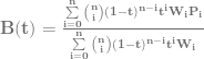

 are the control points and
  are the weightings associated with those control points.
 .
. or
or  or
or  .
. , instead of
  , we come up with the equation in the next section.
 for ANY value
  using the binomial theorem (well, N has to be a positive integer…)





 case. The next row down is “1,2,1” which is the constants multiplied by each term for the
  case. Lastly the next row down (fourth row) is “1,3,3,1” which is the constants multiplied by each term for the
  case. Essentially, you just use the
  th tow of pascals triangle to come up with the constants to multiply each term by.
 , and then multiply each term by a unique control point (A,B,C,etc). After you have your equation, you can optionally replace all
  ‘s with
  , or you can just remember that when you evaluate the equation, since the first form is less messy.


 (Sigma, going from 0 to n) means that you are going to sum (add) together n+1 terms (it includes both 0 and n), using i as the loop variable in your summation. It’s basically a for loop, adding together each iteration of the for loop. Everything that comes after is what happens during each iteration of the for loop that gets summed together.
 part means to take the ith number from the (n+1)th row of Pascal’s triangle. More formally, this specifies to use specific binomial coefficients.
 means that you multiply the binomial coefficient by s to the (n-i)th power, and t to the ith power. This is the same as saying s starts at power n and counts down left to right, while t starts at 0 and counts up left to right. This fits the pattern we saw above in binomial expansion.
 which means to use the ith P. So, P is basically an array with n+1 elements. This array is the control points, so each P is a different control point.




 The blog at the bottom of the sea