This is an extension of a paper I wrote which shows how to use the linear texture sampling capabilities of the GPU to calculate points on Bezier curves. You store the control points in the texture, then sample along the texture’s diagonal to get points on the curve:
GPU Texture Sampler Bezier Curve Evaluation

I’ve been thinking about the items in the “future work” section and found some interesting things regarding polynomials, logic gates, surfaces and volumes. This is the first post, which deals with evaluating polynomials.

Evaluating Polynomials

One of the main points of my paper was that N-linear interpolation (linear, bilinear, trilinear, etc) can be used to evaluate the De Casteljau algorithm since both things are just linear interpolations of linear interpolations. (Details on bilinear interpolation here: Bilinear Filtering & Bilinear Interpolation).

This meant that it was also able to calculate Bernstein Polynomials (aka the algebraic form of Bezier curves), since Bernstein polynomials are equivalent to the De Casteljau algorithm.

I started looking around to see what would happen if you messed around with the De Casteljau algorithm a bit, like interpolate at one level by
or or by a constant or by another variable completely. My hope was that I’d be able to make the technique more generic and open it up to a larger family of equations, so people weren’t limited to just Bernstein polynomials.

That opened up a pretty deep rabbit hole on polynomial blossoming and something called Symmetric Multiaffine Functions. There are some great links in the answer here:
Math Stack Exchange: Modifying and Generalizing the De Casteljau Algorithm

In the end, it turned out to be pretty simple though. It turns out that any polynomial can be converted back and forth from “Power Basis” (which looks like 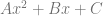) to “Bernstein Basis” (which looks like ) so long as they are the same degree.

This isn’t the result I was expecting but it is a nice result because it’s simple. I think there is more to be explored by sampling off the diagonal, and using different t values at different stages of interpolation, but this result is worth sharing.

By the way, you could also use curve fitting to try and approximate a higher degree function with a lower degree one, but for this post, I’m only going to be talking about exact conversion from Bernstein polynomials to Power polynomials.

Since we can convert power basis polynomials to Bernstein polynomials, and the technique already works for Bernstein polynomials, that means that if we have some random polynomial, say 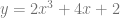, that we can make this technique work for that too. The technique got a little closer to arbitrary equation evaluation. Neat!

Converting Power Basis to Bernstein Basis

I found the details of the conversion process at Polynomial Evaluation and Basis Conversion which was linked to by Math Stack Exchange: Convert polynomial curve to Bezier Curve control points.

This is best explained working through examples, so let’s start by converting a quadratic polynomial from power basis to Bernstein basis.

Quadratic Function

The first thing we do is write the coefficients vertically, starting with the coefficient, then the coefficient and continuing on to the highest value :

Next, we need to divide by the Binomial Coefficients (aka the row of Pascal’s Triangle which has the same number of items as we have coefficients). In this case we need to divide by: 1,2,1.

Now we generate a difference table backwards. it’s hard to explain what that is in words, but if you notice, each value is the sum of the value to the left of it, and the one below that.

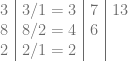
We are all done. The control points for the Bezier curve are on the top row (ignoring the left most column). They are 3,7,13 which makes it so we have the following two equations being equal. The first is in power basis, the second is in Bernstein basis.

Note: don’t forget that Bezier curves multiply the control points by the appropriate row in Pascal’s triangle. That’s where the 14 comes from in the middle term of the Bernstein polynomial. We are multiplying the control points 3,7,13 by the row in Pascal’s triangle 1,2,1 to get the final coefficients of 3,14,13.

Let’s have Wolfram Alpha help us verify that they are equal.

Wolfram Alpha: graph y=2x^2+8x+3, y=3*(1-x)^2+14x*(1-x)+13x^2, from 0 to 1

Yep, they are equal! If you notice the legend of the graph, wolfram actually converted the Bernstein form back to power basis, and you can see that they are exactly equivalent.

You can also write the Bernstein form like the below, which i prefer, using instead of and also setting .

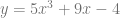
Cubic Function

A cubic function is not that much harder than a quadratic function. After this, you should see the pattern and be able to convert any degree easily.

Again, the first thing we do is write the coefficients vertically, starting with the constant term. Note that we don’t have an term, so it’s coefficient is 0.

We next divide by the Pascal’s triangle row 1,3,3,1.

Now, make the difference table going backwards again:

Our Bezier control points are along the top: -4,-1,2,10. Keeping in mind that the coefficients for a cubic bezier curve are multiplied by 1,3,3,1 we can make the Bernstein form and put it next to our original formula:

Let’s check in wolfram alpha again:
Wolfram Alpha: graph y=5x^3+9x-4, y=-4(1-x)^3-3x(1-x)^2+6x^2(1-x)+10x^3, from 0 to 1

And here it is in the cleaner form:

Some Notes On Calculating Polynomials with the Texture Sampler

You may notice that in the comparison graphs i only plotted the graphs from 0 to 1 on the x axis (aka the t axis). The equations are actually equivalent outside of that range as well, but the technique from my paper only works from the 0 to 1 range because it relies on built in hardware pixel interpolation. This may sound like a big limitation, but if you know the minimum and maximum value of x that you want to plug into your equation at runtime, you can convert your x into a percent between those values, get the resulting polynomial, convert it to Bernstein form, set up the texture, and then at runtime convert your input parameter into that percent when you do the lookup. In other words, you squeeze the parts of the function you care about into the 0 to 1 range.

Another issue you will probably hit is that standard RGBA8 textures have only 8 bits per channel and can only store values between 0 and 1. Since the texture is supposed to be storing your control points, that is bad news.

One way to get around this is to find the largest coefficient value and divide the others by this value. This will put the coefficients into the 0 to 1 range, which will be able to be stored in your texture. After sampling the texture, you multiply the result by that scaling value to get the correct answer.

Scaling won’t help having both negative and positive coefficients though. To handle negative coefficients, you could map the 0-1 space to be from -1 to 1, similar to how we often do it with normal maps and other signed data stored in textures. After doing the lookup you’d have to unmap it too of course.

You could also solve negative values and scaling problems by squishing the y axis into the 0 to 1 space by subtracting the minimum and dividing by the maximum minus the minimum, similarly to how we squished the x range into 0 to 1.

If you instead move to an RGBAF32 texture, you’ll have a full 32 bit float per color channel and won’t have problems with either large values or negative values. You will still have to deal with x only going from 0 to 1 though.

I also want to mention that the hardware texture interpolation works in a X.8 fixed point format. There are more details in my paper, but that means that you’ll get some jagged looking artifacts on your curve instead of a smoothly varying value. If that is a problem for you in practice, my paper talks about a few ways to mitigate that issue.

Before moving on, I wanted to mention that it’s easy to support rational polynomials using this method as well. A rational polynomial is when you divide one polynomial by another polynomial, and relates to rational Bezier curves, where you divide one curve by another curve (aka you give weights to control points). Rational curves are more powerful and in fact you can perfectly represent sine and cosine with a quadratic rational polynomial. More info on that in my paper.

To calculate rational polynomials, you just encode the numerator polynomial in one color channel, and the denominator polynomial in another color channel. After you sample the texture and get the result of your calculation, you divide the numerator value by the denominator value. It costs one division in your shader code, but that’s pretty cheap for the power it gives you!

Regarding the texture size requirements to store a polynomial of a specific degree…

Every dimension of the texture, and every color channel in that texture, adds a degree.

However, to get the benefit of the degree increase from the color channel, you need to do a little more math in the shader – check my paper for more details!

So, if you wanted to store a quadratic polynomial in a texture, you would need either a 2d texture with 1 color channel, or you could do it with a 1d texture that had 2 color channels.

If you wanted to store a cubic polynomial in a texture, you could use a 3d texture with 1 color channel, or a 2d texture with two color channels (there would be some waste here) or a 1d texture with three color channels.

For a polynomial that had a maximum degree term of 6, you could use a 3d volume texture that had 3 color channels: RGB.

If you need to evaluate a very high degree polynomial, you can actually take multiple texture samples and combine them.

For instance, if you had a 2d texture with a single color channel, you could do a single texture read to get a quadratic.

If you did two texture reads, you would have two quadratics.

If you linearly interpolated between those two quadratics, you would end up with a cubic.

That isn’t a very high degree curve but is easier to grasp how they combine.

Taking this up to RGBA 3d volume textures, a single texture read will get you a curve of degree 6. If you do another read, it will take it to degree 7. Another read gets you to 8, another to 9, etc.

With support for 4d textures, an RGBA texture read would give you a degree 7 curve. Another read would boost it to 8, another to 9, another to 10, etc.

Regarding the specific sizes of the textures, in all cases the texture size is “2” on each dimension because we are always just linearly interpolating within a hyper cube of pixel values. You can increase the size of the texture for piecewise curves, check out the paper for more details on that and other options.

Closing

Hopefully you found this useful or interesting!

There may not have been much new information in here for the more math inclined people, but I still think it’s worth while to explicitly show how the technique works for both Bernstein polynomials as well as the more common power basis polynomials.

I still think it would be interesting to look at what happens when you sample off of the diagonal, and also what happens if you use different values at different stages of the interpolation. As an example, instead of just looking up a texture at (t,t) for the (u,v) value to get a quadratic curve point, what if we look up by (t,t^2)? At first blush, it seems like by doing that we may be able to boost a curve to a higher degree, maybe at the cost of some reduced flexibility for the specific equations we can evaluate?

Next up I’ll be writing up some more extensions to the paper involving logic gates, surfaces, and volumes.

Have any feedback, questions or interesting ideas? Let me know!