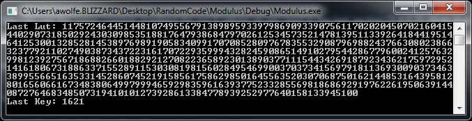
In part 1 (Quantum Computing For Programmers Part I: One Qubit) we looked at the basics of quantum computing and how to deal with a single qubit. Here we’ll talk about the interesting things that happen when you involve multiple qubits!
Multiple Qubit Probabilities & Possibilities
In the last post we used the analogy of a coin to describe a qubit. The coin can be either heads or tails, or flipping in the air, waiting to become either a heads or tails when it lands. The same is true of how a qubit works, where it can either be a 0 or a 1 or some superposition of both, only deciding which it is when observed. Furthermore, just like a real coin, there can be a bias towards becoming one value or the other.
We represented a coin by having a probability for each possible state (heads or tails), but represented a qubit by having an AMPLITUDE for each possible state (0 or 1), where you square an amplitude to get the probability.
Going back to the coin analogy, how would probabilities work if we had two coins?
The four possible outcomes with two coins are:
Heads/Heads
Heads/Tails
Tails/Heads
Tails/Tails
Each coin individually could either be sitting on the table heads or tails, or up in the air, waiting to become either a heads or a tails, with some probability of becoming a heads or a tails.
To figure out the probability of each possible outcome, you just multiply the probability of each coin’s outcome together.
For instance, let’s say that the first coin (coin A) is already sitting on the table as a heads, and the second coin (coin B) is flipping in the air, with a 1/3 chance of becoming heads and a 2/3 chance of becoming tails. Here is how you would calculate the probability of each possible state:

Qubits actually work the same way! Using the same values as the coins, let’s say qubit A is a 0, and qubit B has a 1/3 chance of becoming a 0, and a 2/3 chance of becoming a 1. Converting those probabilities to amplitudes you could get ![A=[1,0], B=[\frac{1}{\sqrt{3}}, \frac{\sqrt{2}}{\sqrt{3}}]](https://s0.wp.com/latex.php?latex=A%3D%5B1%2C0%5D%2C+B%3D%5B%5Cfrac%7B1%7D%7B%5Csqrt%7B3%7D%7D%2C+%5Cfrac%7B%5Csqrt%7B2%7D%7D%7B%5Csqrt%7B3%7D%7D%5D&bg=ffffff&fg=666666&s=0&c=20201002) .
.

Note that in both cases, the probabilities add up to 100% like you’d expect.
In the case of qubits, the resulting vector is ![[\frac{1}{\sqrt{3}}, \frac{\sqrt{2}}{\sqrt{3}}, 0, 0]](https://s0.wp.com/latex.php?latex=%5B%5Cfrac%7B1%7D%7B%5Csqrt%7B3%7D%7D%2C+%5Cfrac%7B%5Csqrt%7B2%7D%7D%7B%5Csqrt%7B3%7D%7D%2C+0%2C+0%5D+&bg=ffffff&fg=666666&s=0&c=20201002) , which is still normalized, and represents the amplitudes for the 4 possible states of those two qubits: 00, 01, 10 and 11.
, which is still normalized, and represents the amplitudes for the 4 possible states of those two qubits: 00, 01, 10 and 11.
When working with one qubit (or coin), there are 2 possible outcomes 0 or 1 (heads or tails). When working with two qubits (or coins), there are four possible outcomes 00, 01, 10, 11 (heads/heads, heads/tails, tails/heads, tails/tails). When working with three qubits or coins, there are eight possible outcomes: 000,001,010 … 111.
With both coins and qubits there are  possibilities, where
  is the number of qubits or coins you have.
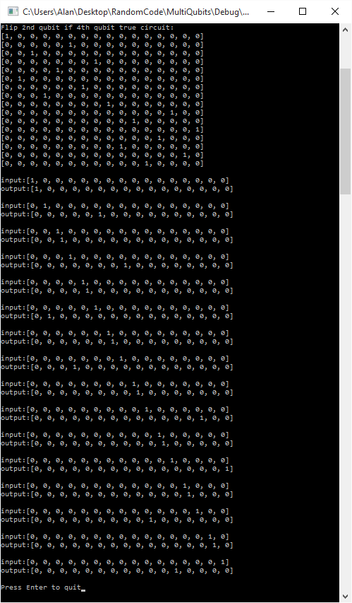
If you had 8 qubits, you’d have to use a 256 dimensional vector to describe the possibilities, since  is 256. When performing quantum computing with 8 qubits, you only have to deal with the 8 qubits. When simulating quantum computing on a regular, classical computer, you have to deal with the 256 amplitudes. This kind of gives a glimpse at how quantum computers can be faster than regular computers at certain things. There is an economy of scale working against us on regular computers simulating quantum computing.
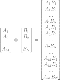
The method we used to combine the probabilities of single qubits into an amplitude vector representing multiple qubits is called the Kronecker product. That’s just a fancy way of saying we have to multiply everything from the first vector by everything from the second vector, to get a third vector that is bigger than the first two. You’ll see it represented like this:  and while it’s similar to the “outer product” and even uses the same symbol (!), it gives a slightly different result versus if you did an outer product and then vectorized the matrix.
The Kronecker product of vectors works like this:
Let’s show an example involving two qubits.
The first qubit has a 75% chance of being heads so it’s amplitude is ![[\sqrt{3}/2,1/2]](https://s0.wp.com/latex.php?latex=%5B%5Csqrt%7B3%7D%2F2%2C1%2F2%5D&bg=ffffff&fg=666666&s=0&c=20201002) . The second qubit has a 2/3 chance of being heads so has an amplitude of
. The second qubit has a 2/3 chance of being heads so has an amplitude of ![[\sqrt{2}/\sqrt{3}, 1/\sqrt{3}]](https://s0.wp.com/latex.php?latex=%5B%5Csqrt%7B2%7D%2F%5Csqrt%7B3%7D%2C+1%2F%5Csqrt%7B3%7D%5D&bg=ffffff&fg=666666&s=0&c=20201002) .
.
To calculate the amplitude vector representing these two qubits, we do a kronecker product:
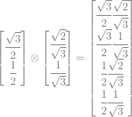
If you simplify that, you get:
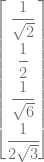
or horizontally for easier reading:

Squaring those values to get the probabilities of each state, we get the below, which you might notice adds up to 100%, meaning the vector is still normalized!

This generalizes for larger numbers of qubits, so you could use the Kronecker product to combine a vector describing 4 qubits with a vector describing 3 qubits, to come up with a vector that describes 7 qubits (which would have 128 amplitudes in it, since 2^7 = 128!).
The kronecker product also generalizes to matrices, which we will talk about shortly.
To be able to work with multiple qubits in a quantum circuit, you need to represent all qubits involved in a single vector. Doing this, while being the correct thing to do, also allows entanglement to happen, which we will talk about next!
Entanglement – Simpler Than You Might Think!
Time to demystify quantum entanglement!
Quantum entanglement is the property whereby two qubits – which can be separated by any distance, such as several light years – can be observed and come up with the same value (0 or 1). Whether they are 0s or 1s is random, but they will both agree, when entangled in the way that causes them to agree (you could alternately entangle them to always disagree).
Interestingly, in 1965 John Bell proved that the mechanism that makes this happen is NOT that the qubits share information in advance. You can read more about that here – it’s near the end: Ars Technica – A tale of two qubits: how quantum computers work.
A common misconception is that this means that we can have faster than light (instantaneous) communication across any distance. That turns out not to be true, due to the No-Communication-Theorem (Wikipedia).
Interestingly though, you can use separated entangled qubits in separated quantum circuits to do something called Quantum Pseudo Telepathy (Wikipedia), which lets you do some things that would otherwise be impossible – like reliably winning a specially designed game that would otherwise be a game of chance.
I don’t yet understand enough about Quantum Pseudo Telepathy to see why it isn’t considered communication. I also have no idea how entanglement is actually “implemented” in the universe, but nobody seems to (or if they do, they aren’t sharing!). How can it be that two coins flipped on opposite sides of the galaxy can be guaranteed to both land with the same side facing up?
Despite those mysteries, the math is DEAD SIMPLE, so let me share it with you, it’ll take like one short paragraph. Are you ready?
Quantum computing works by manipulating the probabilities of the states of qubits. If you have two qubits, there are four possible sets of values when you observe them: 00, 01, 10, 11. If you use quantum computing to set the probabilities of the 01 and 10 states to a 0% chance, and set the probabilities of the 00 and 11 states to a 50% chance each, you’ve now entangled the qubits such that when you observe them, they will always agree, because you’ve gotten rid of the chances that they could ever DISAGREE. Similarly, if instead of setting the 01 and 10 states to 0%, you set the probability of the 00 and 11 states to 0%, you’d have entangled qubits which would always disagree when you observed them, because you’ve gotten rid of the chances that they could ever AGREE.
That’s all there is to it. Strange how simple it is, isn’t it? The table below shows how the only possible outcomes are that the qubits agree, but it is a 50/50 chance whether they are a 0 or a 1:

Entanglement isn’t limited to just two qubits, you can entangle any number of qubits together.
Entanglement has a special mathematical meaning. If you can represent a state of a group of qubits by a kronecker product, they are not entangled. If you CAN’T represent a state of a group of qubits by a kronecker product, they ARE entangled. These two things – entanglement and lack of kronecker product factorability (made that term up) – are the same thing.
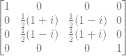
As an example, what two vectors could you use the kronecker product on to get the entangled two qubit state  (or in vector form
 ![[1/\sqrt{2}, 0, 0, 1/\sqrt{2}]](https://s0.wp.com/latex.php?latex=%5B1%2F%5Csqrt%7B2%7D%2C+0%2C+0%2C+1%2F%5Csqrt%7B2%7D%5D&bg=ffffff&fg=666666&s=0&c=20201002) )? You’ll find there aren’t any! That state is the entangled state where the two qubits will always have the same value when you observe them.
)? You’ll find there aren’t any! That state is the entangled state where the two qubits will always have the same value when you observe them.
Entangled qubits are nothing special in quantum circuits. You don’t have to take any special precautions when working with them. They are an interesting byproduct of quantum computing, and so basically are something neat that comes out of your quantum circuit, but they don’t require any extra thought when using them within your circuits. Don’t worry about them too much (:
Multi Qubit Gates
Let’s have a look at some multi qubit gates! (These are again from Wikipedia: Quantum Gate)
Swap Gate
Given two qubits, with possible states 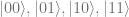 , this gate swaps the amplitudes (probabilities) of
  and leaves the probabilities of the states
  and
and  alone.
That might seem weird, but the probability of the state is the probability of the first qubit being 0 added to the probability of the second qubit being 0. If those probabilities swap, they still add to the same value, so this probability is unaffected. It’s the same situation for the state.
Here’s the matrix for the swap gate:

Square Root of Swap Gate
I don’t really understand a usage case for this gate myself, but it apparently does a half way swap between two qubits. That once again modifies the probabilities of the states, but leaves state and alone again, for the same reason as the swap gate.
Wikipedia says that if you have this gate, and the single qubit gates, that you can do universal quantum computation. In other words, you can build a fully functional quantum computer using just this and the single qubit gates.
Here’s the matrix:
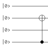
Controlled Not Gate
The controlled not (CNOT) gate flips the value of the second qubit if the first qubit is true. This is a logic / flow control type of gate.
Interestingly, this gate is also useful for creating entangled qubits, which you’ll be able to see lower down!
Here is the matrix:

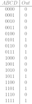
The controlled not gate is also referred to as the quantum XOR gate. To see why, check out the truth table below for this gate:

If you look at the right most bit of the outputs, you’ll notice that it’s the XOR of the two input bits!
All quantum gates need to be reversible, and having these two qubits be the output of a hypothetical quantum XOR gate allows that to happen. If you look at the right most bit of the inputs, you’ll notice that it is also the XOR of the two output bits. It’s bidirectional, which is kind of weird and kind of interesting 😛
Generalized Control Gate
You can actually convert any single qubit gate into a controlled gate. That makes a 2 qubit gate which only does work on the second qubit if the first qubit is true.
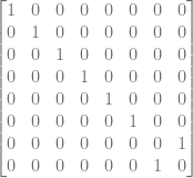
How you do that is you make a 4×4 identity matrix, and make the lower 2×2 sub-matrix into the single qubit matrix you want to use.
In other words, if your single qubit matrix is this:

Then the controlled version of the matrix would be this:

Pretty simple right?
Toffoli Gate
The Tofolli gate is a 3 qubit gate that is also known as the CCNOT gate or controlled controlled not gate. It flips the third qubit if the first two qubits are true.
It’s matrix looks pretty uninteresting:
This is also known as the quantum AND gate. If you look at the truth table below, you’ll see that when the input has the right most qubit of 0, that in the output, the right most qubit will be the AND value of the two left qubits. We need the three bits of input mapping to three bits of output like this so that the gate is reversible.

Fredkin Gate
The Fredkin gate is a controlled swap gate. Here’s the matrix:

Just like we talked about how to make a generalized controlled gate acting on two qubits, you should be able to notice that this gate is just a specific version of a generalized controlled 3 qubit gate. You take an 8×8 identity matrix, and make the lower right 4×4 matrix be the 2 qubit gate that you want to add a control on. In this case, the lower right 4×4 matrix is just the swap gate we mentioned earlier in the post (:
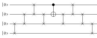
Circuit To Entangle Qubits
The circuit to entangle qubits is pretty simple, so let’s start with that as the first quantum circuit we look at. It takes in two qubits. The first qubit is put through a Hadamard gate, and then both qubits are put through a controlled not gate. That circuit looks like this (image courtesy of Quantum Circuit Simulator):
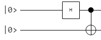
The value you plug in for the second qubit determines what type of entanglement you get out. Setting the second qubit to 0, you will get entangled qubits which always agree when they are observed. Setting it to 1, you will get entangled qubits which always disagree when they are observed. The first qubit controls whether the phase of each state matches or mismatches. Note that these are the four Bell States (Wikipedia: Bell State).
![\begin{array}{c|c|c} \text{Input} & \text{Output In Ket Notation} & \text{Output As Vector} \\ \hline 00 & \frac{1}{\sqrt{2}}(|00\rangle+|11\rangle) & [1/\sqrt{2},0,0,1/\sqrt{2}] \\ 01 & \frac{1}{\sqrt{2}}(|01\rangle+|10\rangle) & [0,1/\sqrt{2},1/\sqrt{2},0] \\ 10 & \frac{1}{\sqrt{2}}(|00\rangle-|11\rangle) & [1/\sqrt{2},0,0,-1/\sqrt{2}] \\ 11 & \frac{1}{\sqrt{2}}(|01\rangle-|10\rangle) & [0,1/\sqrt{2},-1/\sqrt{2},0]\\ \end{array}](https://s0.wp.com/latex.php?latex=%5Cbegin%7Barray%7D%7Bc%7Cc%7Cc%7D+%5Ctext%7BInput%7D+%26+%5Ctext%7BOutput+In+Ket+Notation%7D+%26+%5Ctext%7BOutput+As+Vector%7D+%5C%5C+%5Chline+00+%26+%5Cfrac%7B1%7D%7B%5Csqrt%7B2%7D%7D%28%7C00%5Crangle%2B%7C11%5Crangle%29+%26+%5B1%2F%5Csqrt%7B2%7D%2C0%2C0%2C1%2F%5Csqrt%7B2%7D%5D+%5C%5C+01+%26+%5Cfrac%7B1%7D%7B%5Csqrt%7B2%7D%7D%28%7C01%5Crangle%2B%7C10%5Crangle%29+%26+%5B0%2C1%2F%5Csqrt%7B2%7D%2C1%2F%5Csqrt%7B2%7D%2C0%5D+%5C%5C+10+%26+%5Cfrac%7B1%7D%7B%5Csqrt%7B2%7D%7D%28%7C00%5Crangle-%7C11%5Crangle%29+%26+%5B1%2F%5Csqrt%7B2%7D%2C0%2C0%2C-1%2F%5Csqrt%7B2%7D%5D+%5C%5C+11+%26+%5Cfrac%7B1%7D%7B%5Csqrt%7B2%7D%7D%28%7C01%5Crangle-%7C10%5Crangle%29+%26+%5B0%2C1%2F%5Csqrt%7B2%7D%2C-1%2F%5Csqrt%7B2%7D%2C0%5D%5C%5C+%5Cend%7Barray%7D+&bg=ffffff&fg=666666&s=0&c=20201002)
In a quantum circuit, you can’t just apply a gate to an individual quabit at a time though. You have to make the matrix of your gate such that it applies to all qubits, applying the “identity” matrix to the qubits you don’t want to be affected by the gate.
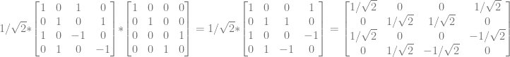
So, how do we make a matrix that applies the Hadamard gate to qubit 1, and identity to qubit 2? You use the kronecker product!
Since we want to apply the Hadamard matrix to qubit 1 and identity to qubit 2, we are going to calculate  (If we wanted to apply the Hadamard gate to qubit 2 and identity to qubit 1 we would calculate
  instead).

If you notice, the result of the kronecker product is just every value in the left matrix, multiplied by every value in the right matrix. Basically, the result is a 2×2 grid of identity matrices, where each of those identity matrices is multiplied by the corresponding value from the same cell in the left matrix. Since the left matrix has a 1 in all cells except the lower right, the same is true of the result… it’s a positive identity matrix in each cell, except the lower right one, which is a negative identity matrix. Hopefully that makes sense, it’s a lot easier than it sounds…
The second gate in the quantum circuit is the CNOT gate. We can actually multiply the gate we just made by the CNOT gate to represent the full quantum circuit as a single matrix. This uses regular matrix multiplication.
Lets plug some values into the circuit and see what comes out!
Lets start by plugging in 00. Our input qubits are ![[1, 0]](https://s0.wp.com/latex.php?latex=%5B1%2C+0%5D&bg=ffffff&fg=666666&s=0&c=20201002) and . The kronecker product of those two qubit vectors is
and . The kronecker product of those two qubit vectors is ![[1, 0, 0, 0]](https://s0.wp.com/latex.php?latex=%5B1%2C+0%2C+0%2C+0%5D&bg=ffffff&fg=666666&s=0&c=20201002) . Now let’s multiply that vector by the matrix of our quantum circuit.
. Now let’s multiply that vector by the matrix of our quantum circuit.

Comparing this to the table showing how our input maps to output, we got the right answer! If you plugged in the other values listed, you would get the rest of the bell state entanglements.
Unentangling Qubits
All gates are reversible, so all circuits are reversible. To get the reverse circuit for a given matrix, you just get the inverse of the matrix. Since quantum gates (and circuits) are unitary matrices, taking the inverse of one of these matrices just means taking the conjugate transpose of the matrix. In other words, you take the transpose of the matrix, and then just negate the imaginary component of any complex numbers. In this example, there are no imaginary numbers, so you just take the transpose of the matrix.
Since our circuit matrix is this:

That means that the inverse must be this, since this is the (conjugate) transpose.

Let’s try it out by putting the output from last section in and seeing what comes out the other side:

It worked! We got our original input back.
Making Matrices for More Complex Circuits
We talked about how to make single qubit gates apply to specific qubits by using the kronecker product with identity to move the gate to the right location.
If you have 4 qubits and you want to apply some single qubit gate (say Hadamard) to the 3rd qubit, you would just do this to get the matrix:
What if you want to do complex things with multi qubit gates though? Like what if you want to do a controlled not gate where you want the 2nd qubit to flip it’s value if the 4th qubit was true?
The answer is actually pretty simple… you use swaps gates to flip the values of the qubits so that your qubit values line up with the inputs of the gate, then you do the gate, and finally undo all the swaps to get the qubit values back to the right positions.
We need to swap qubits so that the 4th qubit value is in the 1st qubit slot, and the 2nd qubit value is in the 2nd qubit slot. We can do that with the following swaps:
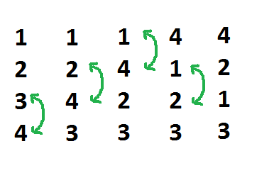
Once we have done those swaps, we can do our controlled not, then do the swaps in reverse order to return the qubits to their original positions.
Here’s what the circuit looks like:
You’ll see the simpler version in circuit diagrams, but at least now you’ll know how to make things that look like this:
Below is the mathematical way that you would get the matrix representing this gate.
 is the identity matrix,
  is the swap gate, and
  is the controlled not gate.
Code
Here is some simple C++ to show both the entanglement circuit and the more complicated controlled not gate we described.
#include <stdio.h>
#include <vector>
#include <complex>
#include <assert.h>
typedef std::complex<float> TComplex;
//=================================================================================
struct SComplexVector
{
public:
TComplex& Get (size_t i) { return v[i]; }
const TComplex& Get (size_t i) const { return v[i]; }
size_t Size() const
{
return v.size();
}
void Resize (size_t s)
{
v.resize(s);
}
void Print () const
{
printf("[");
for (size_t i = 0, c = v.size(); i < c; ++i)
{
if (i > 0)
printf(", ");
const TComplex& val = Get(i);
if (val.imag() == 0.0f)
{
if (val.real() == 0.0f)
printf("0");
else if (val.real() == 1.0f)
printf("1");
else
printf("%0.2f", val.real());
}
else
printf("%0.2f + %0.2fi", val.real(), val.imag());
}
printf("]n");
}
std::vector<TComplex> v;
};
//=================================================================================
struct SComplexMatrix
{
public:
TComplex& Get (size_t x, size_t y)
{
return v[y*Size() + x];
}
const TComplex& Get (size_t x, size_t y) const
{
return v[y*Size() + x];
}
// For an MxM matrix, this returns M
size_t Size () const
{
size_t ret = (size_t)sqrt(v.size());
assert(ret*ret == v.size());
return ret;
}
// For an MxM matrix, this sets M
void Resize(size_t s)
{
v.resize(s*s);
}
void Print() const
{
const size_t size = Size();
for (size_t y = 0; y < size; ++y)
{
printf("[");
for (size_t x = 0; x < size; ++x)
{
if (x > 0)
printf(", ");
const TComplex& val = Get(x, y);
if (val.imag() == 0.0f)
{
if (val.real() == 0.0f)
printf("0");
else if (val.real() == 1.0f)
printf("1");
else
printf("%0.2f", val.real());
}
else
printf("%0.2f + %0.2fi", val.real(), val.imag());
}
printf("]n");
}
}
std::vector<TComplex> v;
};
//=================================================================================
static const SComplexVector c_qubit0 = { { 1.0f, 0.0f } }; // false aka |0>
static const SComplexVector c_qubit1 = { { 0.0f, 1.0f } }; // true aka |1>
// 2x2 identity matrix
static const SComplexMatrix c_identity2x2 =
{
{
1.0f, 0.0f,
0.0f, 1.0f,
}
};
// Given the states |00>, |01>, |10>, |11>, swaps the |01> and |10> state
// If swapping the probabilities of two qubits, it won't affect the probabilities
// of them both being on or off since those add together. It will swap the odds of
// only one of them being on.
static const SComplexMatrix c_swapGate =
{
{
1.0f, 0.0f, 0.0f, 0.0f,
0.0f, 0.0f, 1.0f, 0.0f,
0.0f, 1.0f, 0.0f, 0.0f,
0.0f, 0.0f, 0.0f, 1.0f
}
};
// Controlled not gate
// If the first qubit is true, flips the value of the second qubit
static const SComplexMatrix c_controlledNotGate =
{
{
1.0f, 0.0f, 0.0f, 0.0f,
0.0f, 1.0f, 0.0f, 0.0f,
0.0f, 0.0f, 0.0f, 1.0f,
0.0f, 0.0f, 1.0f, 0.0f
}
};
// Hadamard gate
// Takes a pure |0> or |1> state and makes a 50/50 superposition between |0> and |1>.
// Put a 50/50 superposition through and get the pure |0> or |1> back.
// Encodes the origional value in the phase information as either matching or
// mismatching phase.
static const SComplexMatrix c_hadamardGate =
{
{
1.0f / std::sqrt(2.0f), 1.0f / std::sqrt(2.0f),
1.0f / std::sqrt(2.0f), 1.0f / -std::sqrt(2.0f)
}
};
//=================================================================================
void WaitForEnter ()
{
printf("nPress Enter to quit");
fflush(stdin);
getchar();
}
//=================================================================================
SComplexVector KroneckerProduct (const SComplexVector& a, const SComplexVector& b)
{
const size_t aSize = a.Size();
const size_t bSize = b.Size();
SComplexVector ret;
ret.Resize(aSize*bSize);
for (size_t i = 0, ic = aSize; i < ic; ++i)
{
for (size_t j = 0, jc = bSize; j < jc; ++j)
{
size_t n = i * bSize + j;
ret.Get(n) = a.Get(i)*b.Get(j);
}
}
return ret;
}
//=================================================================================
SComplexMatrix KroneckerProduct (const SComplexMatrix& a, const SComplexMatrix& b)
{
const size_t aSize = a.Size();
const size_t bSize = b.Size();
SComplexMatrix ret;
ret.Resize(aSize*bSize);
for (size_t ax = 0; ax < aSize; ++ax)
{
for (size_t ay = 0; ay < aSize; ++ay)
{
const TComplex& aValue = a.Get(ax, ay);
for (size_t bx = 0; bx < bSize; ++bx)
{
for (size_t by = 0; by < bSize; ++by)
{
const TComplex& bValue = b.Get(bx, by);
size_t nx = ax*bSize + bx;
size_t ny = ay*bSize + by;
ret.Get(nx,ny) = aValue * bValue;
}
}
}
}
return ret;
}
//=================================================================================
SComplexMatrix operator* (const SComplexMatrix& a, const SComplexMatrix& b)
{
assert(a.Size() == b.Size());
const size_t size = a.Size();
SComplexMatrix ret;
ret.Resize(size);
for (size_t nx = 0; nx < size; ++nx)
{
for (size_t ny = 0; ny < size; ++ny)
{
TComplex& val = ret.Get(nx, ny);
val = 0.0f;
for (size_t i = 0; i < size; ++i)
val += a.Get(i, ny) * b.Get(nx, i);
}
}
return ret;
}
//=================================================================================
SComplexVector operator* (const SComplexVector& a, const SComplexMatrix& b)
{
assert(a.Size() == b.Size());
const size_t size = a.Size();
SComplexVector ret;
ret.Resize(size);
for (size_t i = 0; i < size; ++i)
{
TComplex& val = ret.Get(i);
val = 0;
for (size_t j = 0; j < size; ++j)
val += a.Get(j) * b.Get(i, j);
}
return ret;
}
//=================================================================================
int main (int argc, char **argv) {
// 2 qubit entanglement circuit demo
{
// make the circuit
const SComplexMatrix H1 = KroneckerProduct(c_hadamardGate, c_identity2x2);
const SComplexMatrix circuit = H1 * c_controlledNotGate;
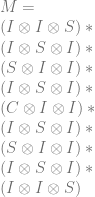
// display the circuit
printf("Entanglement circuit:n");
circuit.Print();
// permute the inputs and see what comes out when we pass them through the circuit!
SComplexVector input = KroneckerProduct(c_qubit0, c_qubit0);
SComplexVector output = input * circuit;
printf("ninput:");
input.Print();
printf("output:");
output.Print();
input = KroneckerProduct(c_qubit0, c_qubit1);
output = input * circuit;
printf("ninput:");
input.Print();
printf("output:");
output.Print();
input = KroneckerProduct(c_qubit1, c_qubit0);
output = input * circuit;
printf("ninput:");
input.Print();
printf("output:");
output.Print();
input = KroneckerProduct(c_qubit1, c_qubit1);
output = input * circuit;
printf("ninput:");
input.Print();
printf("output:");
output.Print();
}
// 4 qubit demo: flip the second qubit if the fourth qubit is true
{
// make the circuit
const SComplexMatrix cnot4qubit = KroneckerProduct(KroneckerProduct(c_controlledNotGate, c_identity2x2), c_identity2x2);
const SComplexMatrix swap12 = KroneckerProduct(KroneckerProduct(c_swapGate, c_identity2x2), c_identity2x2);
const SComplexMatrix swap23 = KroneckerProduct(KroneckerProduct(c_identity2x2, c_swapGate), c_identity2x2);
const SComplexMatrix swap34 = KroneckerProduct(KroneckerProduct(c_identity2x2, c_identity2x2), c_swapGate);
const SComplexMatrix circuit =
swap34 *
swap23 *
swap12 *
swap23 *
cnot4qubit *
swap23 *
swap12 *
swap23 *
swap34;
// display the circuit
printf("nFlip 2nd qubit if 4th qubit true circuit:n");
circuit.Print();
// permute the inputs and see what comes out when we pass them through the circuit!
SComplexVector input = KroneckerProduct(KroneckerProduct(KroneckerProduct(c_qubit0, c_qubit0), c_qubit0), c_qubit0);
SComplexVector output = input * circuit;
printf("ninput:");
input.Print();
printf("output:");
output.Print();
input = KroneckerProduct(KroneckerProduct(KroneckerProduct(c_qubit0, c_qubit0), c_qubit0), c_qubit1);
output = input * circuit;
printf("ninput:");
input.Print();
printf("output:");
output.Print();
input = KroneckerProduct(KroneckerProduct(KroneckerProduct(c_qubit0, c_qubit0), c_qubit1), c_qubit0);
output = input * circuit;
printf("ninput:");
input.Print();
printf("output:");
output.Print();
input = KroneckerProduct(KroneckerProduct(KroneckerProduct(c_qubit0, c_qubit0), c_qubit1), c_qubit1);
output = input * circuit;
printf("ninput:");
input.Print();
printf("output:");
output.Print();
input = KroneckerProduct(KroneckerProduct(KroneckerProduct(c_qubit0, c_qubit1), c_qubit0), c_qubit0);
output = input * circuit;
printf("ninput:");
input.Print();
printf("output:");
output.Print();
input = KroneckerProduct(KroneckerProduct(KroneckerProduct(c_qubit0, c_qubit1), c_qubit0), c_qubit1);
output = input * circuit;
printf("ninput:");
input.Print();
printf("output:");
output.Print();
input = KroneckerProduct(KroneckerProduct(KroneckerProduct(c_qubit0, c_qubit1), c_qubit1), c_qubit0);
output = input * circuit;
printf("ninput:");
input.Print();
printf("output:");
output.Print();
input = KroneckerProduct(KroneckerProduct(KroneckerProduct(c_qubit0, c_qubit1), c_qubit1), c_qubit1);
output = input * circuit;
printf("ninput:");
input.Print();
printf("output:");
output.Print();
input = KroneckerProduct(KroneckerProduct(KroneckerProduct(c_qubit1, c_qubit0), c_qubit0), c_qubit0);
output = input * circuit;
printf("ninput:");
input.Print();
printf("output:");
output.Print();
input = KroneckerProduct(KroneckerProduct(KroneckerProduct(c_qubit1, c_qubit0), c_qubit0), c_qubit1);
output = input * circuit;
printf("ninput:");
input.Print();
printf("output:");
output.Print();
input = KroneckerProduct(KroneckerProduct(KroneckerProduct(c_qubit1, c_qubit0), c_qubit1), c_qubit0);
output = input * circuit;
printf("ninput:");
input.Print();
printf("output:");
output.Print();
input = KroneckerProduct(KroneckerProduct(KroneckerProduct(c_qubit1, c_qubit0), c_qubit1), c_qubit1);
output = input * circuit;
printf("ninput:");
input.Print();
printf("output:");
output.Print();
input = KroneckerProduct(KroneckerProduct(KroneckerProduct(c_qubit1, c_qubit1), c_qubit0), c_qubit0);
output = input * circuit;
printf("ninput:");
input.Print();
printf("output:");
output.Print();
input = KroneckerProduct(KroneckerProduct(KroneckerProduct(c_qubit1, c_qubit1), c_qubit0), c_qubit1);
output = input * circuit;
printf("ninput:");
input.Print();
printf("output:");
output.Print();
input = KroneckerProduct(KroneckerProduct(KroneckerProduct(c_qubit1, c_qubit1), c_qubit1), c_qubit0);
output = input * circuit;
printf("ninput:");
input.Print();
printf("output:");
output.Print();
input = KroneckerProduct(KroneckerProduct(KroneckerProduct(c_qubit1, c_qubit1), c_qubit1), c_qubit1);
output = input * circuit;
printf("ninput:");
input.Print();
printf("output:");
output.Print();
}
WaitForEnter();
return 0;
}
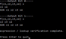
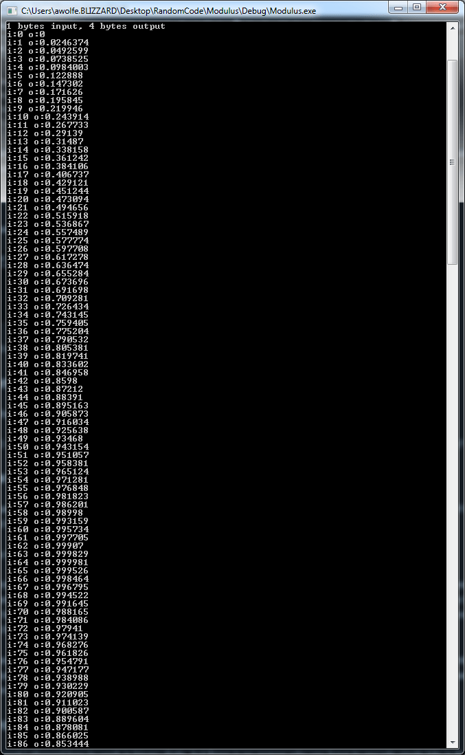
Here is the first part of the output, which shows the results of the entangling circuit. You can see that the input gave the expected output Bell states:
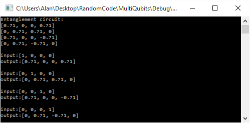
Below is the second part of the output, which is the circuit that flips the 2nd qubit if the 4th qubit is true.
Each entry in the input and output vectors is the amplitude (probability) that the state it represents is true. The states start at the left with 0000, then 0001, then 0010 and continue until the very right most value which represents 1111.
If you look at the second input/output pair the input is [0,1,0,0,0,0,0,0,0,0,0,0,0,0,0,0], which means it has a 100% chance of the 4 qubits being 0001 (aka the qubits represent the number 1). The output vector is [0,0,0,0,0,1,0,0,0,0,0,0,0,0,0,0], which means that it has a 100% chance of being 0101 (aka the qubits represent the number 5). Since the input did have the 4th bit set (4th from the left), it flipped the 2nd bit. So, you can see that it worked!
If you check all the input/output pairs, you’ll see that they all follow this rule.
We used only whole, real numbers, no using fractional probabilities, or imaginary amplitudes. What it does in those situations is a little bit harder to get intuition for, but rest assured that it does “the right thing” in those situations as well.
Next Up
Now that we have the basics of quantum computing down pretty well, it’s time to analyze a couple quantum algorithms to see how they work!


 different pieces, where if you have any
  of those
  in that equation, but use your secret number as the constant term.
 aka
aka  . Those are your shares. You then give individual shares to people, or go hide them in your dungeon or do whatever you are going to do with them.
 .
.

 values are random numbers, and
  is the secret value.


 and instead of shares being
  . In technical terms we are going to be using points on a finite field, or a Galois field.
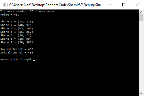


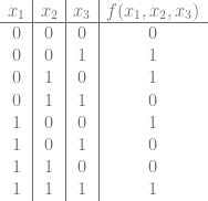


 , we just look in the truth table for function
  to see if we have an odd or even number of ones in the output of the function. If there is an even number, it is 0, else it is a 1.
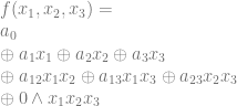
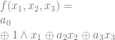
 is the symbol for AND. I’m showing it explicitly because otherwise the equation looks weird, and a multiplication symbol isn’t correct.
 , we need to limit our truth table to
  . That truth table is below, made from the original truth table, but throwing out any row where
  is 1.
is 1.

 , we find that it also has an even number of ones, making
  become 0 and making that term disappear.
 , it also has an even number of ones, making
  become 0 and making that term disappear as well.
 , we look at the truth table for
  , which is below:

 and
and  , you’ll find that they also have odd numbers of ones in the output so also become ones. That puts our equation at:
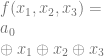
 , is just looking at whether there are an odd or even number of ones in the function
  which you can look up directly in the lookup table. It’s even, so


 , and all the other identities to help you simplify equations.


 are involved in our group, so
  is not involved in any places where there is a 1, so we can ignore that too. All that leaves is
  , which is our final, and most minimal answer.
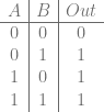


 as an answer, which in other words is just A OR B. Check out the truth table and you can see that it is indeed a truth table for OR!
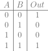

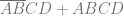
 , while the lower right group is expressed as
  . We OR those two groups together to get the answer:
  . That’s all there is to it.


 , which is also the answer:


 and
and  are the values that we modulus x against to get our desired outputs out.


 ) be the OR of the input bits and the right output bit (
 ) be the AND of the input bits.

 where n is an integer. Fermat numbers also have the benefit that you can get the nth item in the list without calculating the numbers that came before it. The only problem is that the numbers grow super huge very fast. The first 7 values are: 3, 5, 17, 257, 65537, 4294967297, 18446744073709551617. If Fermat numbers didn’t grow so quickly, they sure would be useful for things like this technique.
![[0.5,0.5]](https://s0.wp.com/latex.php?latex=%5B0.5%2C0.5%5D&bg=ffffff&fg=666666&s=0&c=20201002)
![[0.75,0.25]](https://s0.wp.com/latex.php?latex=%5B0.75%2C0.25%5D&bg=ffffff&fg=666666&s=0&c=20201002)
 .
.![[1/\sqrt{2}, 1/\sqrt{2}]](https://s0.wp.com/latex.php?latex=%5B1%2F%5Csqrt%7B2%7D%2C+1%2F%5Csqrt%7B2%7D%5D&bg=ffffff&fg=666666&s=0&c=20201002) .
.![[\sqrt{3}/2, 1/2]](https://s0.wp.com/latex.php?latex=%5B%5Csqrt%7B3%7D%2F2%2C+1%2F2%5D&bg=ffffff&fg=666666&s=0&c=20201002) . If you square the first number you can see that you get 3/4 (75% chance) and squaring the second number gives you 1/4 (25% chance).
. If you square the first number you can see that you get 3/4 (75% chance) and squaring the second number gives you 1/4 (25% chance).
 is the desired probability from 0 to 1.


![[-1/\sqrt{2}, 1/\sqrt{2}]](https://s0.wp.com/latex.php?latex=%5B-1%2F%5Csqrt%7B2%7D%2C+1%2F%5Csqrt%7B2%7D%5D&bg=ffffff&fg=666666&s=0&c=20201002)
![[1/\sqrt{2}, 1/\sqrt{2}] + [1/\sqrt{2}, 1/\sqrt{2}] = [\sqrt{2}, \sqrt{2}]](https://s0.wp.com/latex.php?latex=%5B1%2F%5Csqrt%7B2%7D%2C+1%2F%5Csqrt%7B2%7D%5D+%2B+%5B1%2F%5Csqrt%7B2%7D%2C+1%2F%5Csqrt%7B2%7D%5D+%3D+%5B%5Csqrt%7B2%7D%2C+%5Csqrt%7B2%7D%5D+&bg=ffffff&fg=666666&s=0&c=20201002)
 state has opposite phase in one of the vectors:
![[1/\sqrt{2}, 1/\sqrt{2}] + [1/\sqrt{2}, -1/\sqrt{2}] = [\sqrt{2}, 0]](https://s0.wp.com/latex.php?latex=%5B1%2F%5Csqrt%7B2%7D%2C+1%2F%5Csqrt%7B2%7D%5D+%2B+%5B1%2F%5Csqrt%7B2%7D%2C+-1%2F%5Csqrt%7B2%7D%5D+%3D+%5B%5Csqrt%7B2%7D%2C+0%5D+&bg=ffffff&fg=666666&s=0&c=20201002)
![[1/\sqrt{2}, 1/\sqrt{-2}]](https://s0.wp.com/latex.php?latex=%5B1%2F%5Csqrt%7B2%7D%2C+1%2F%5Csqrt%7B-2%7D%5D&bg=ffffff&fg=666666&s=0&c=20201002)
![[1/\sqrt{2}, 1/(\sqrt{2}*i)]](https://s0.wp.com/latex.php?latex=%5B1%2F%5Csqrt%7B2%7D%2C+1%2F%28%5Csqrt%7B2%7D%2Ai%29%5D&bg=ffffff&fg=666666&s=0&c=20201002)
![[0,i]](https://s0.wp.com/latex.php?latex=%5B0%2Ci%5D&bg=ffffff&fg=666666&s=0&c=20201002) , if you square the
, if you square the  state to get the probability, you get -1, or -100%. That isn’t right!
 , the complex conjugate is
  .
. by
by  to get 1, or 100%.
 state to
  and
and  .
.


 ends up being a complex number, that can also be written like this:
 is any angle in radians.
![[1/\sqrt{2}, -1/\sqrt{2}]](https://s0.wp.com/latex.php?latex=%5B1%2F%5Csqrt%7B2%7D%2C+-1%2F%5Csqrt%7B2%7D%5D&bg=ffffff&fg=666666&s=0&c=20201002) which has opposite phases for each state.
which has opposite phases for each state.
 , as well as in Shor’s algorithm, which can factor large numbers much faster than classical computers, putting certain types of cryptography at risk for being cracked by quantum computers.
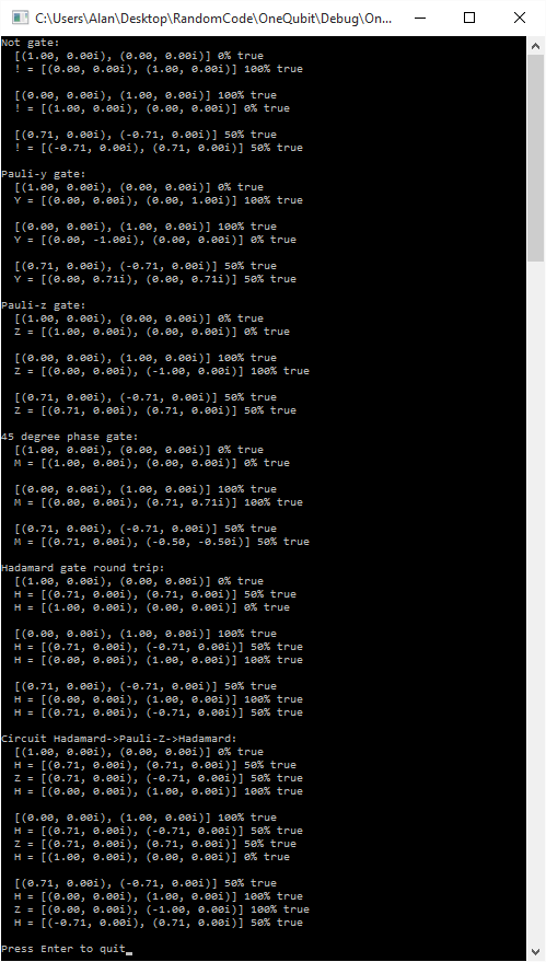


 where
where  .
. where
where  .
. which reads as “in all integers mod 2”.
 .
. where
where  and
and 
 where
where 


![a = [1,3]](https://s0.wp.com/latex.php?latex=a+%3D+%5B1%2C3%5D&bg=ffffff&fg=666666&s=0&c=20201002)
 ,
,  ,
, ![b = [1,3,6]](https://s0.wp.com/latex.php?latex=b+%3D+%5B1%2C3%2C6%5D&bg=ffffff&fg=666666&s=0&c=20201002)


 where N is any integer, aka
  .
.


 , it will always be a perfect multiple of 3 and 11, which means that the value will be zero in the other terms / other equations, so won’t affect whatever value we come up for them.
 .
. where
where  , but we can stick to using 15 to make it easier to follow.


 where
where 
