The last post showed how random Hamiltonian cycles on a graph (a path that visits each node exactly once) could efficiently handle ranking of a large number of items, by doing sparse pairwise voting (https://blog.demofox.org/2023/09/01/sparse-pairwise-voting-or-tournaments-implementing-some3-voting/).

That algorithm needed to generate multiple Hamiltonian cycles which didn’t use any graph edges already used by other cycles, and I didn’t like that it did this by generating cycles randomly until it found one that is valid. The “randomly generate candidates until success” meant an erratic runtime that might not even find a solution in a reasonable amount of time.

This post shows a way to generate those cycles in a straightforward way and compares the resulting cycles to the algorithm in the previous post. The algorithm requires a prime number count of nodes, but if you don’t have a prime number count of nodes, you can pad the graph with extra nodes to make it reach the next prime number. If the cycles are for voting, you can make those padding nodes automatically lose to real nodes, without needing to do an actual vote. This algorithm also works with non prime number amounts of nodes if you relax what “works” means a bit; instead of making cycles, it will sometimes make isolated loops, but we talk about how that can still be useful.

The code that goes with this post lives at https://github.com/Atrix256/PairwiseVoting. The visual “star” diagrams were made with drawgraphs.py. The csv files for the graphs were made by main.cpp.

The Algorithm

The algorithm is pretty straightforward.

If you have N nodes and N is a prime number, you loop from 0 to N-1. nodeA is the loop index. nodeB is (nodeA + 1) % N. This is the first cycle.

For the second cycle, you loop again. nodeA is the loop index. nodeB is (nodeA + 2) % N.

For the third cycle, you loop again. nodeA is the loop index. nodeB is (nodeA + 3) % N.

To get all cycles, you repeat this, for each integer from 1 to N/2, but not including N/2.

Let’s see an example.

Example 1 – Five Nodes

For the first cycle, we use each node index 0,1,2,3,4 as nodeA, and add 1 to each, modulo 5, to get nodeB.

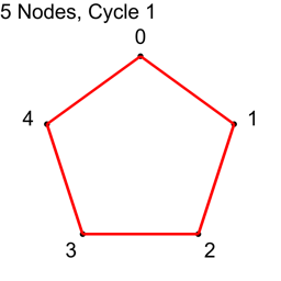
We next add 2:

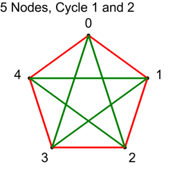
N/2 is 2.5, so we should stop at this point. Let’s see what happens if we do 3 anyways.

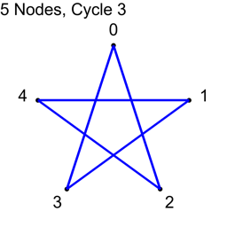
We got the same connections when we added 3, as when adding 2. We’ll see why shortly.

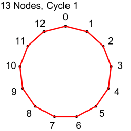
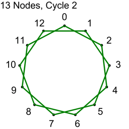
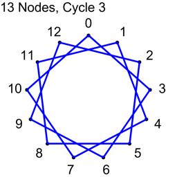
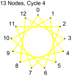
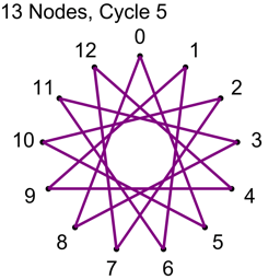
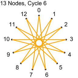
Example 2 – Thirteen Nodes

Just the diagrams, one cycle at a time, because otherwise it’s too messy.

Why Does This Work?

For the first cycle, we start with every node we have as nodeA, then add 1 and modulo by N to get each nodeB. That gives us N connections, and they are all unique. We have used up all the connections where the nodes are 1 index apart and no other cycle is going to make a connection with nodes that are 1 index apart. We know that this is a cycle and that we can get from any node to any other node because you can subtract 1 or add 1 repeatedly to get from any index to any other index.

For the second cycle, we do the same but add 2 and modulo by N to get nodeB. We again have N connections and they are all unique. We also have used up all the connections where the nodes are 2 indices apart and no other cycle is going to make any connection where the nodes are 2 indices apart.

For the second cycle, we can also get from any node to any other node in this cycle, but it’s less obvious why. When working with the integers modulo N, you have something called a ring, which is a type of group. If you start at any number on the ring, and repeatedly add some number M which is relatively prime to N (no common factors other than 1), you will visit all numbers 0 to N-1, and will visit them all once before repeating any. When N is a prime number, then EVERY number less than N is relatively prime to N.

You can try this yourself:

1. Pick some prime number N
2. Pick any number M between 1 and N-1.
3. Starting at zero (or any other value), add M, modulo by N, and write out the value.
4. Repeat step 3 and you’ll see that you’ll visit all N numbers and after N steps you will get back to where you started.

Let’s do this with N=7 and M=2:

So, when N is prime, every time we add a specific value greater than 0 and less than N to all the node indices, we’ll get a cycle that uses edges that no other cycle will give us.

Why Start Cycles at 1 and Stop at N/2?

There are two explanations for why this is. One is a mathematical explanation and the other is a brick wall. Let’s look at the brick wall first, then talk about the mathematical reason.

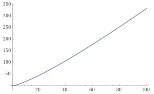
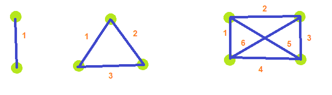
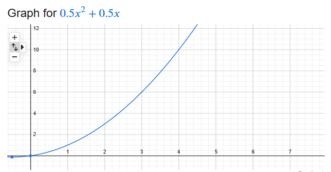
If you have N nodes in a graph, the total number of connections you can make between nodes is N * (N-1) / 2. Tangent: if you think that looks like Gauss’ formula, you are correct! It’s Gauss’ formula for N-1.

Returning to example 1, that had 5 nodes which means there are 5*4/2 = 10 total connections.

Each Hamiltonian cycle on that graph takes 5 connections away from all possible connections, and with 10 connections total, that means there can only be 2 cycles.

5/2 is 2.5, so we do cycle 1, then cycle 2, and stop before we do cycle 3.

We literally cannot do more than 2 cycles when there are 5 nodes.

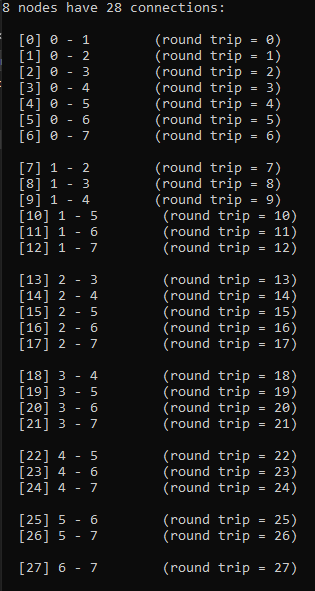
Looking at example 2, there are 13 nodes, which means there are 78 total connections.

Each cycle takes 13 connections, so all connections are used up after 6 cycles.

13/2 is 6.5, so we know to stop at 6 before going to 7.

The brick wall limitation is that after N/2 cycles, we have no more edges to make cycles out of!

The mathematical explanation involves rings. To quote the previous section: When working with the integers modulo N, you have something called a ring, which is a type of group.

In rings, there is an interesting connection between the numbers less than N/2 and the numbers greater than N/2. Adding a number greater than N/2 is the same as subtracting a number less than N/2. As an example, let’s look at N=7 in the table below. We can see that adding 5 is the same as subtracting 2.

This means that if we have a connection where nodeB = (nodeA + 5) % 7, it is exactly the same as the connection where nodeA = (nodeB + 2) % 7. More plainly, cycle 5 will make the same connections as cycle 2. The nodeA and nodeB values will be swapped, but it will be the same connections.

Cycle N/2 is the point where positive numbers become the same as smaller negative numbers, so that is where we stop. Since all prime numbers (greater than 2) are odd, N/2 will never be an integer, so we don’t have to think about what to do at exactly N/2.

What if N isn’t Prime?

If N isn’t prime, not all “cycles” will be cycles. The algorithm will visit all nodes, but there will not be a path from each node to every other node. Here are the cycles for where N=9.

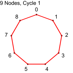
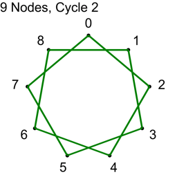
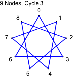
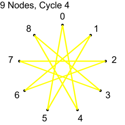
With N=9, only cycles 1,2 and 4 make cycles. Cycle 3 makes three loops: 0,3,6 and 1,4,7 and 2,5,8. If you wanted to use this algorithm to make connections in a graph for voting or for a tournament, you could still do so, but the first cycle you do should be a coprime (cycle 1 is an easy one to choose as the first cycle), so that the graph was connected from the beginning, and these loops would increase connectivity of the graph, without having to be fully fledged Hamiltonian cycles.

Allowing N not to be prime also allows an even numbered N. In that case, when you create cycles from 1 to N/2, should you include N/2 or not? Let’s see what happens when N=6, for cycles 1,2 and 3.

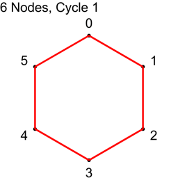
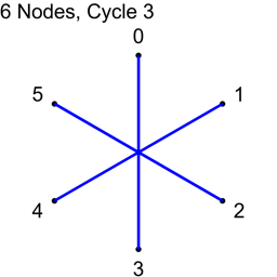
What happened to cycle 3?

Cycle 3 made all the connections where the difference between the node indices was 3, and it made 6 connections. Unfortunately, there are only 3 unique connections where the difference in node indices is 3: 0-3, 1-4, 2-5. Cycle 3 added the following redundant connections: 3-0, 4-1, 5-2. The answer about whether you should include N/2 if using a non prime number of nodes is ultimately up to you, but you should know that when you do so, you’ll get redundant connections. On the flip side, if you don’t include them, those are node connections that you will never be able to make otherwise, using this algorithm. You’ll have to decide which way you want to go. You could always pad with another node to make it odd, and dodge this issue 🙂

Is This Random Enough?

When you see that the first cycle gives you the connections in order 0 – 1, 1 – 2, 2 – 3, etc. you may wonder if this method is making random enough cycles.

In defense of this seeming lack of randomness, keep in mind that node indices are just arbitrary names of nodes. Two nodes that have an index difference of 1 are not any more, or less, similar than two other nodes that have an index difference of 5. The numbers are just arbitrary labels.

However, the lack of randomness does come up on subsequent cycles. Think of the path from node A to node B on graphs made this way as a simplified path finding problem. After you’ve done 1 cycle, you know you can take steps of size 1 from any node to any other node. After you’ve done 2 cycles, you know you can take steps of size 2. After 3 cycles you can take steps of size 3 and so on. Using this knowledge, you can craft a path from A to B using the largest steps to get as close as possible, then a smaller step as a remainder. This is nice and orderly, but when graph edges are taken at random, there will be shortcuts sprinkled throughout the graph. Like if in the first cycle of a 1000 node graph, if there is a link from node 0 to node 500, that will drastically reduce the length of the path between the most distant nodes.

So on one hand, the lack of randomness doesn’t matter, but on another hand, it does.

There are some ways to inject randomness into this algorithm if you want to though. One easy thing you can do is shuffle the nodes before running this algorithm. Another thing you can do is perform the cycles in a random order. If you have 1009 nodes, that gives you 1009/2=504 cycles. The last post showed that you only need a handful of cycles to get a good result if using cycles for voting or tournaments. Instead of doing cycles 1, 2, and 3, you could randomize the order and do it an order like 100, 4, 235. These points of randomization could help make up for lack of randomization in the cycles themselves, and are also helpful if you ever need multiple sets of non overlapping Hamiltonian cycles. That allows this algorithm to take in a “random seed” to get different results for different seeds, while remaining deterministic.

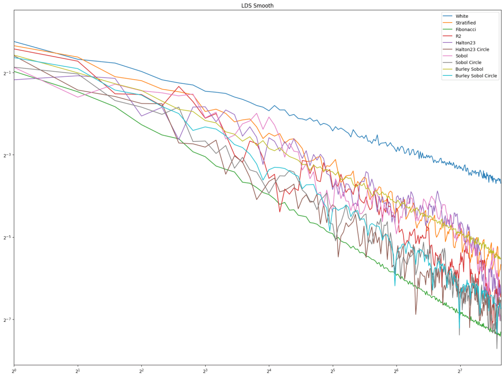
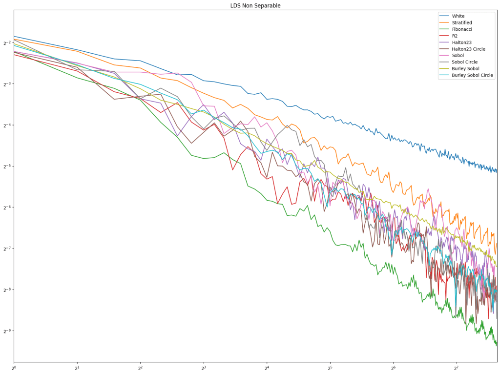
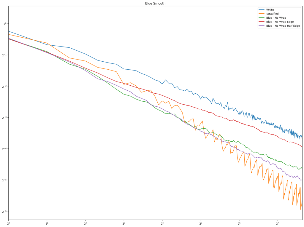
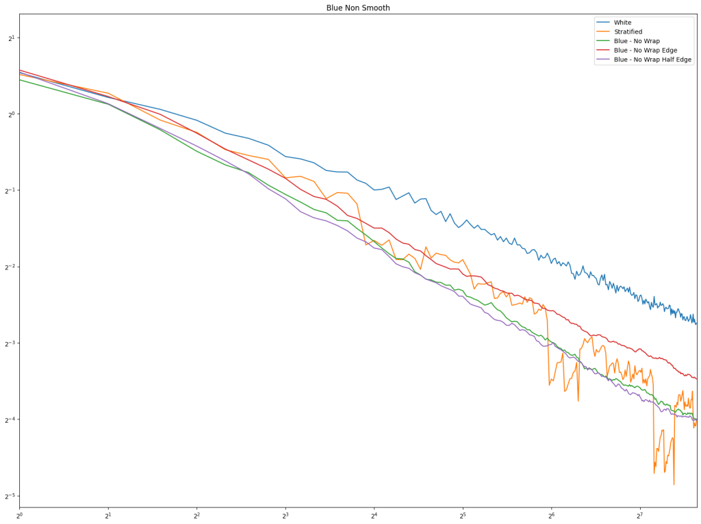
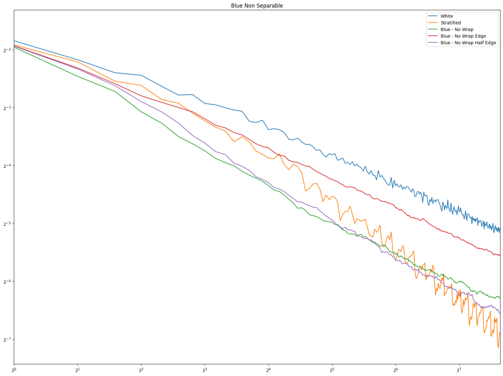
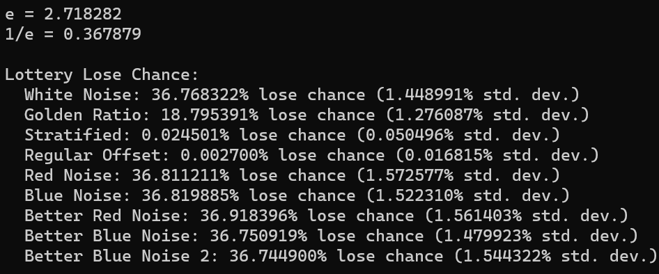
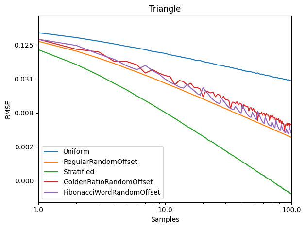
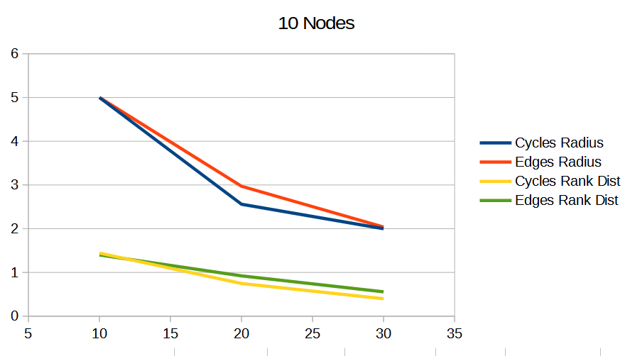
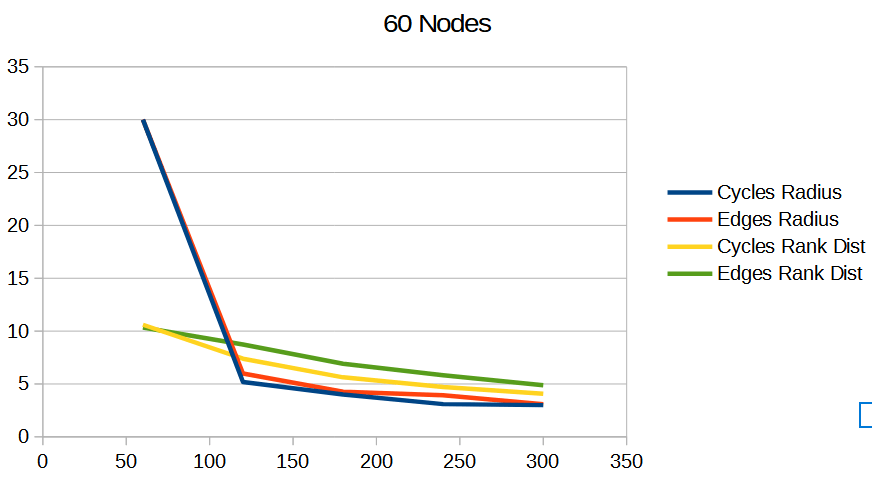
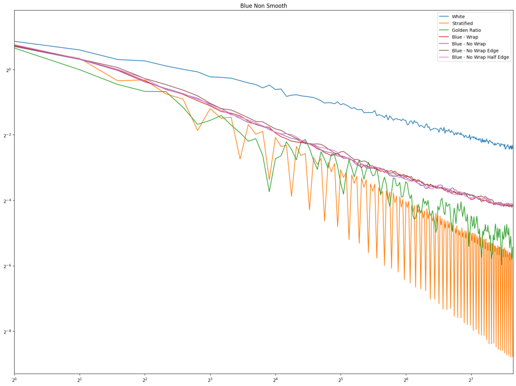
Results In Graph Quality Tests

To understand the quality of these Hamiltonian cycles, I plugged them into the voting algorithm from the last blog post. I put in a version that does cycles in order (1, 2, 3 and so on), and also put in a version that does the cycles in a random order, but makes sure the first cycle is always 1, to ensure the graph is connected, in case the number of nodes is not prime.

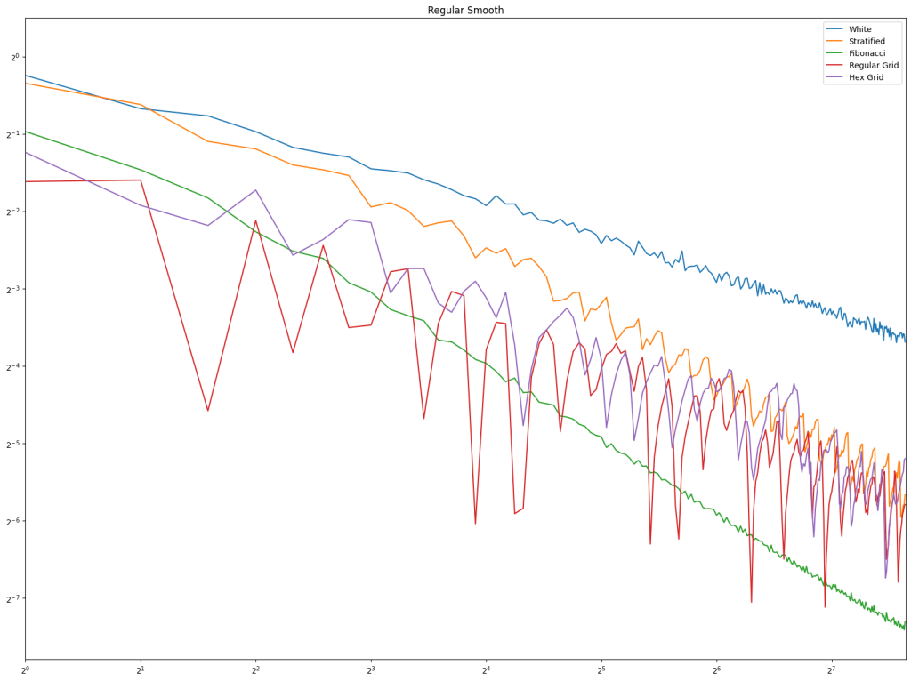
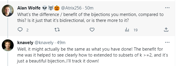
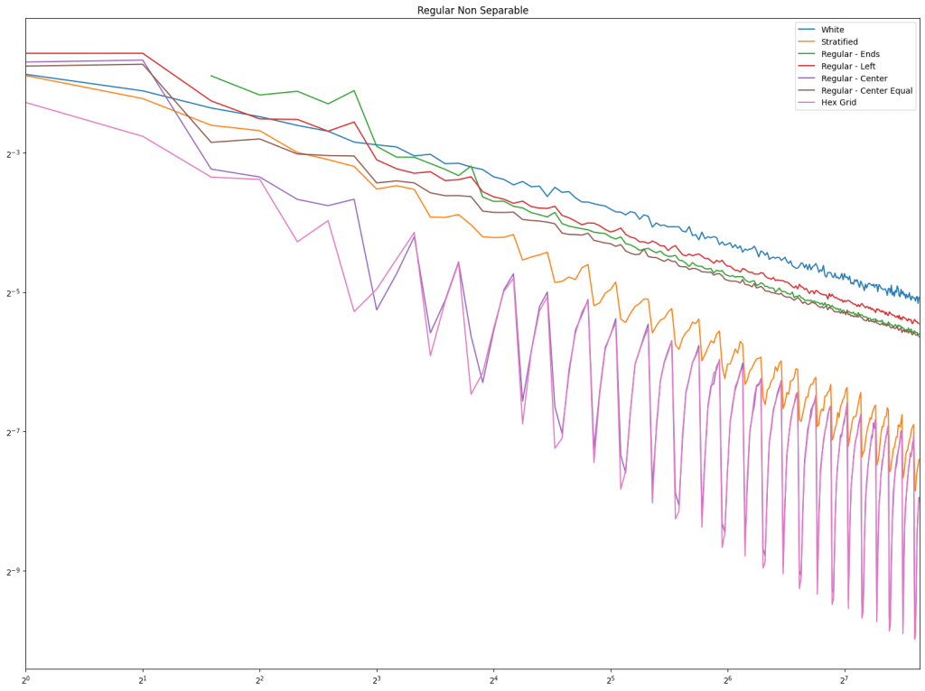
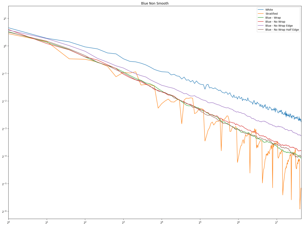
The graphs below are the average of 100 tests. The source code generates csv files with more information, including standard deviation.

For radius, cycles are randomly generated and rings shuffled are shuffled differently each run. The non shuffled rings are the same each test. For rank distance, the actual score value of each node changes each test, so all rank distance graphs are subject to randomization in each test. This can also be seen as shuffling the nodes before running the algorithm, which is sometime I talked about in the last section.

For both radius and rank distance, a lower score is better.

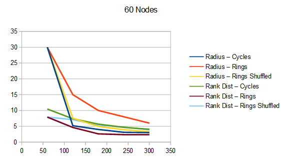
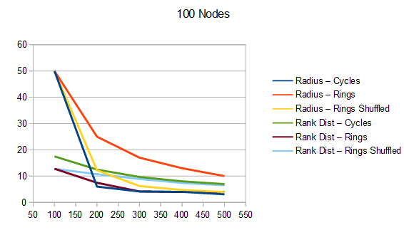
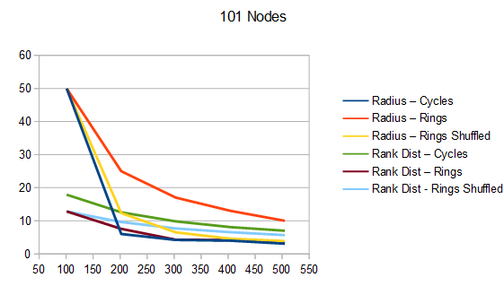
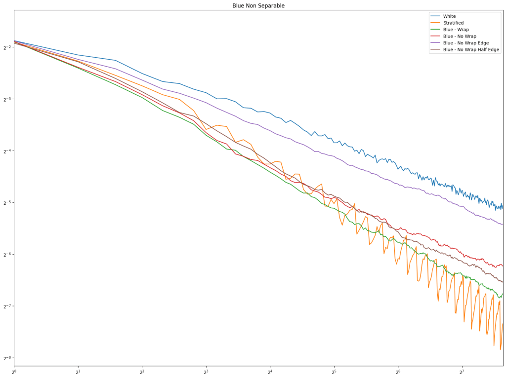
It looks like random cycles (the technique from the last post) decreases the radius the most. That is not surprising, since that is based on solid mathematics to reduce the radius quickly. Using the deterministic cycles in this post, but shuffling the order the cycles looks to be a pretty good method for reducing radius too. It isn’t as good as random cycles, but it can quickly and easily find as many non overlapping Hamiltonian cycles as you want, up to the full limit of how many cycles are possible. Randomly generating cycles until they are valid gets very slow for high cycle counts and high node counts.

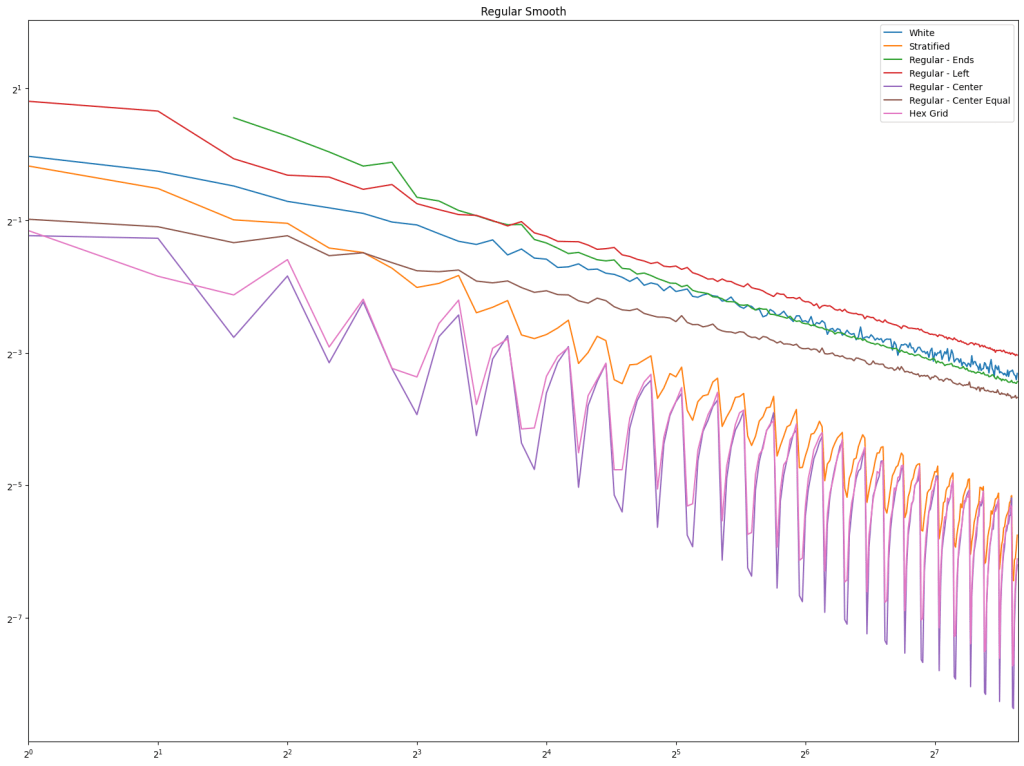
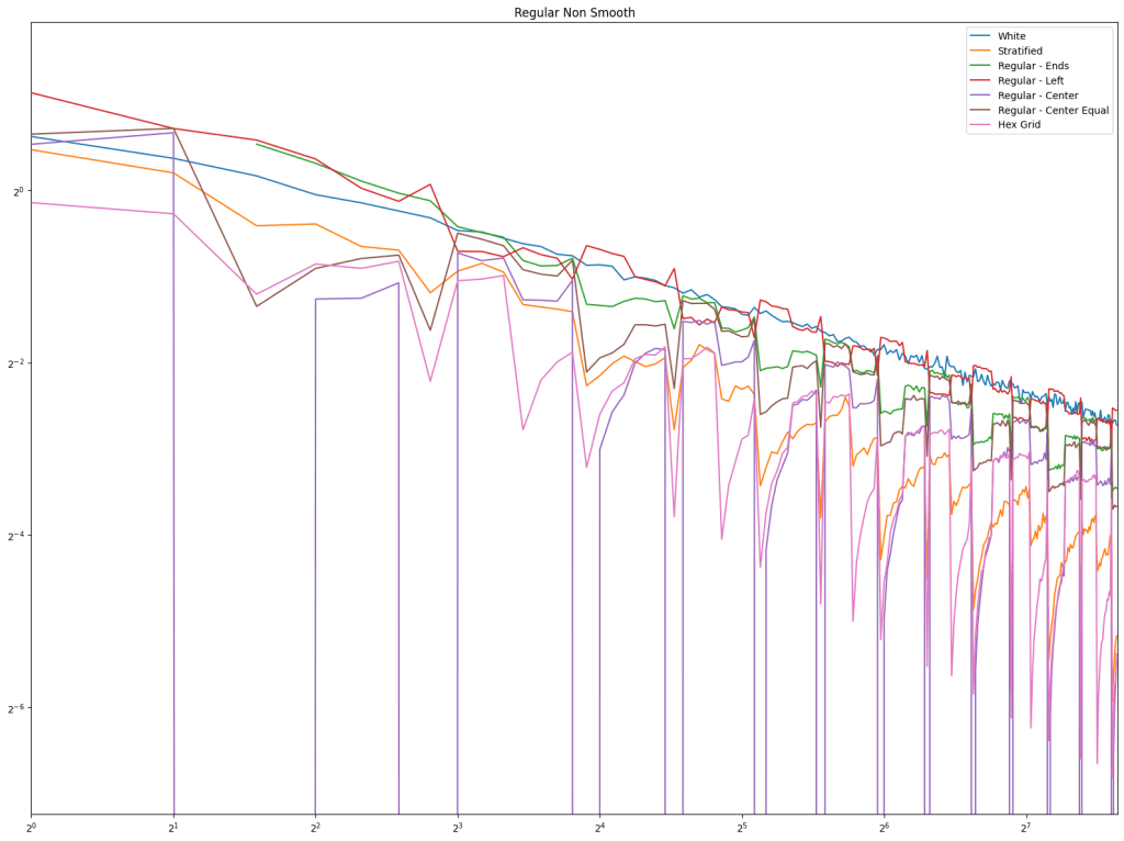
These graphs tell a different story for the rank distance. These show that the NON SHUFFLED ordering of deterministic cycles do the best for making the most accurate ranked list. I’m a bit surprised, as this shows that decreasing radius may be a good idea for improving the ranked list quality, but it isn’t the whole story for making the highest quality ranked list approximation.

Perhaps this has something to do with radius being measured as the worst outlier, while the rank distance is calculated as an average quality of all nodes.

Quick recap on rank distance: The rank distance is calculated by using the voting algorithm from last post to make a ranked list, and then summing up the difference of each node’s placement in that estimated ranking list, versus the nodes placement in the actual ranking list. It’s the optimal transport cost to change the estimated ranking list into the actual ranking list. That value is divided by the number of nodes to try and normalize it.

Anyhow, thanks for reading and thanks to this video by CQFD for nerd sniping me with graph theory 🙂
https://www.youtube.com/watch?v=XSDBbCaO-kc

The C++ code that goes with this blog post is at https://github.com/Atrix256/PairwiseVoting/

There is a great video on YouTube (https://www.youtube.com/watch?v=XSDBbCaO-kc) that explains how voting was implemented in the third Summer of Math Exposition (https://some.3b1b.co/) from 3 Blue 1 Brown (https://www.youtube.com/@3blue1brown).

In the Summer of Math Exposition, people make online math content, and prizes are given to the winners. The challenge is there are thousands of entrants, where a typical entry may be a 30 minute video of nontrivial mathematics. How could all those entries be judged to find the best ones?

The video I linked before talks about how to approach this with graph theory and makes use of a lot of really interesting math, including eigenvectors of adjacency matrices. The result is that they have volunteer judges do a relatively small number of votes between pairs of videos, and from that, the winners emerge in a way that is strongly supported by solid mathematics.

I recommend giving that video a watch, but while the motivation of the technique is fairly complicated, the technique itself ends up being very simple to implement.

I’ll give some simplified background to the algorithm, then talk about how to implement it, and finally show some results.

Background

Let’s assume there are N players in a tournament, where there is an absolute ordering of the players. This is in contrast to rock, paper, scissors, where there is no 1st place, 2nd place, and 3rd place for those three things. We are going to assume that there are no cycles, and the players can actually be ordered from best to worst.

A way to find the ordering of the N players could be to take every possible pair of players A and B and have them play against each other. If we did this, we’d have a fully connected graph of N nodes, and could use an algorithm such as Page Rank (https://en.wikipedia.org/wiki/PageRank) to turn the results of that into an ordered list.

If there are N players, we can use Gauss’ Formula (https://blog.demofox.org/2023/08/21/inverting-gauss-formula/) to calculate that there are N * (N-1) / 2 matches that would need to be played. For 1000 players, that means 499,500 matches. Or in the case of SoME3 videos, that is 499,500 times a volunteer judge declares which is better between two 30 minute math videos. That is a lot of video watching!

Tom Scott has an interesting video about this way of voting: https://www.youtube.com/watch?v=ALy6e7GbDRQ. In that situation, it was just an A/B vote between concepts like “bees” and “candy”, so was a lot quicker to make pairwise votes.

Wouldn’t it be nicer if we could do a smaller number of votes/matches, and do a sparse number of the total votes, while still getting an as accurate result as possible?

The SoME3 video explains how to do this and why the method works.

One thing the video talks about is the concept of a “radius of a graph”.

If you have a node A and a node B, the shortest path on the graph between those nodes is the distance. If you calculate that distance for all nodes, the largest value you get is the radius of the graph.

It’s also important that there is a path between every node to every other node! This is known as the graph being “connected”. If the graph isn’t connected, the radius is undefined since the largest distance will be infinite (no path between 2 nodes). If the radius is 1, such that there is a connection between each node to every other node, then the graph is called a complete graph.

The video talks about how it is important to make the radius smaller for a higher quality result of the voting. The larger the distance between two nodes, the less direct the comparison is between those two nodes which makes their ordering less certain. The shorter the distance, the more direct the comparison is, which makes their ordering more certain. Reducing the graph radius ensures that all distances are smaller or equal to that radius in distance.

You can imagine that if you were to pick pairs to vote on at random, that it probably isn’t going to be the optimal voting pairs to give the smallest radius of a graph. For instance, due to the nature of uniform random numbers, you might have 20 votes between node 5 and other nodes, while you only have 2 votes between node 4 and other nodes. A node picked at random is more likely to have a shorter path to node 5 than it is to node 4, and so node 4 is going to be the longer distance that defines the overall radius of the graph. If the votes were more evenly spread to all the nodes, the maximum distance (aka radius) would go down more.

The Algorithm

The algorithm ends up being super simple:

1. Visit all nodes in a random order. This is a random cycle or a random Hamiltonian cycle.
2. Each connection between nodes in that cycle are votes to be done or matches to be played. So for N nodes, there are N votes. Note that each node is involved in 2 votes, but it’s still only N votes!
3. That is one iteration. Goto 1 again, but when generating a random cycle, make sure it doesn’t contain any edges (votes) already done in a previous iteration. Repeat until you are satisfied.

A simple way to implement visiting all nodes in a random order is to just shuffle a list of integers that go from 0 to N-1.

The magic is that each iteration decreases the radius exponentially.

So, it’s very simple and effective.

Alternate Algorithm

I spent some time thinking about this algorithm and trying to come up with alternatives.

One thing that bothered me was generating random cycles, but making sure no edges in the cycle were already used. That loop may take a very long time to execute. Wouldn’t it be great if there was some O(1) constant time algorithm to get at least a pseudorandom cycle that only contained edges that weren’t visited yet? Maybe something with format preserving encryption to do constant time shuffling of non overlapping cycles?

Unfortunately, I couldn’t think of a way.

Another thought I had was that it would be nice if there was some way to make a “low discrepancy sequence” that would give a sequence of edges to visit to give the lowest radius, or nearly lowest radius for the number of edges already visited.

I also couldn’t think of a way to do that.

For that second idea, I think you could probably brute force calculate a list like that in advance for a specific number of nodes. Once you did it for 10 node graphs, you’d always have the list.

I didn’t pursue that, but it might be interesting to try some day. I would use the radius as the measurement to see which edge would be best to add next. Before the graph is connected, with a path from every node to every other node, the radius is undefined, but that is easily solved by just having the first N edges be from node i to i+1 to make the graph connected.

In the end, I came up with an algorithm that isn’t great but has some nice properties, like no looping on random outcomes.

1. The first iteration makes N connections, connecting each node i to node i+1. This isn’t randomized, but you could shuffle the nodes before this process if you wanted randomized results after this first iteration.
2. Each subsequent iteration makes N new connections. It chooses those N connections (graph edges) randomly, by visiting all N*(N-1)/2 edges in a shuffled, random order. It uses format preserving encryption to make a shuffle iterator with random access, instead of actually shuffling any lists. It knows to ignore any connection between nodes that are one index apart, since that is already done in step 1.

The end result is that the algorithm essentially makes a simple loop for the first iteration, and then picks N random graph edges to connect in each other iteration.

An important distinction between my algorithm and the original is that after the first iteration, the links chosen don’t form a cycle. They are just random links, so may involve some nodes more often and others less often, making for uneven node distances, and larger graph radius values.

Because of this, you could call the SoME3 algorithm a “random cycles” algorithm, and mine a “random edges” algorithm.

Once You Have the Graph…

Whichever algorithm you use makes you end up with a connected graph where the edges between vertices represent votes that need to be done (or matches that need to be played).

When you do those matches, you make the connections be directed instead of undirected. You make the loser point to the winner.

You can then do the page rank algorithm, which makes it so rank flows from losers to winners through those connections to get a final score for each node. You can sort these final scores to get a ranking of nodes (players, videos, whatever) that is an approximation of the real ranking of the nodes.

In the code that goes with this post, I gave each node a “random” score (hashing the node id) and that score was used to determine the winner in each edge, by comparing this score between the 2 nodes involved to find which one won.

Since each node has an actual score, I was able to make an actual ranking list to compare to the approximated one.

We now need a way to compare how close the approximated ranking list is, compared to the actual ranking list. This tells us how good our approximation is.

For this, I summed the absolute value of the actual rank of a node minus the approximated rank of a node, for all nodes. If my thinking is correct, this is equivalent to optimal transport and the 1-Wasserstein distance, which seems like the appropriate metric to use here (more info: https://blog.demofox.org/2022/07/27/calculating-the-similarity-of-histograms-or-pdfs-using-the-p-wasserstein-distance/).

I divided this sum by the number of nodes to normalize it a bit, but graphs of different sizes still had slightly different scale scores.

Results

Below are some graphs comparing the random cycles algorithm (“Cycles”) to the random edges algorithm (“Edges”). The radius is the radius of the graph, and lower is better. The rank dist says how accurate the approximated rank was, and lower is better.

The graphs show that the random cycles algorithm does better than the random edges algorithm, both in radius, as well as accuracy of the approximated ranking.

Frankly, each iteration being a random hamiltonian cycle on a graph has a certain “low discrepancy” feel to it, compared to random edge selection which feels a lot more like uniform random sampling. By choosing a random cycle, you are making sure that each node participates in 2 votes or matches each iteration. With random edge selection, you are making no such guarantee for fairness, and that shows up as worse results.

To me, that fairness / “low discrepancy” property is what makes choosing random cycles the superior method.

In the graphs below, the x axis is the number of votes done. Each data point is at an iteration. The graphs show the average of 100 tests.

What About Tournament Brackets?

Tournament brackets are another way of finding a winner by having pairwise votes or matches.

If you have 8 players, you pair them up and play 4 matches to get 4 winners. You then pair them up to get 2 matches and 2 winners. Lastly you play the last match to get the winner. That is 4+2+1=7 matches for players.

If you have 16 players, you first do 8 matches, then 4 matches, then 2 matches, then 1 match. That is 8+4+2+1=15 matches for 16 players.

In general, If you have N items, it only takes N-1 votes or matches to get a winner – and assuming matches have no random chance in them, gives you the EXACT winner. In the SoME3 algorithm, each iteration takes N votes or matches, and there are multiple iterations, so seems to take a lot more votes or matches.

That is true, and tournament brackets are very efficient at finding the winner by doing pairwise comparisons.

Tournament brackets can only tell you who is first and who is second though. They can’t tell you who is third. They can tell you who made it to the finals or semi finals etc, but the people who made it to those levels have no ordering within the levels.

Another factor to consider is that who plays in a tournament match depends on who won the previous matches. This makes it so later matches are blocked from happening until earlier matches have happened.

If these things aren’t a problem for your situation, a tournament bracket is pretty efficient with matches and votes! Otherwise, you might reach for the SoME3 algorithm 🙂

What About Merge Sort?

Leonard Ritter aka paniq (https://mastodon.gamedev.place/@lritter) brought up this excellent point on mastodon.

So interestingly, merge sort is a lot like tournament brackets, where the earlier matches define who plays in the later matches. However, the number of matches played in total can vary!

Lets say you had two groups of four players, where in each group, you knew who was best, 2nd best, 3rd best and last. And say you wanted to merge these two groups into one group of eight, knowing who was best, 2nd best, etc all the way to last.

The merge operation of merge sort (https://www.youtube.com/watch?v=4VqmGXwpLqc) would do between 4 and 7 comparisons here to get that merged list, which is between 4 and 7 matches or votes for us. If you then wanted to merge two groups of 8, it would do between 8 and 15 comparisons.

In general, if you have N items, the fewest number of comparisons merge sort will do is N/2 * log2(N). This is each merge will at minimum do N comparisons, and there are log2(N) levels of merging.

The graph for that is pretty linear which is nice. No large growth of comparisons as the number of items or nodes grow. This is what makes merge sort a decent sorting algorithm.

Ultimately, this connection shows that the SoME3 voting algorithm can also be seen as an approximate sorting algorithm, which is neat.

Links

Here are some links I found useful in understanding the Page Rank algorithm:
https://en.wikipedia.org/wiki/PageRank
https://www.ccs.neu.edu/home/vip/teach/IRcourse/4_webgraph/notes/Pagerank%20Explained%20Correctly%20with%20Examples.html
https://towardsdatascience.com/pagerank-algorithm-fully-explained-dc794184b4af

This post has an interesting link to the last one (Inverting Gauss’ Formula). The last post was focused on adding all the numbers from 1 to N, this post will feature multiplying all the numbers from 1 to N.

We aren’t going to be doing it in constant time though, if you want that check out this page: https://devblogs.microsoft.com/oldnewthing/20151214-00/?p=92621.

Calculating The Number of Permutations

Let’s say we have 3 letters A,B,C. How many ways are there to arrange them?

If you look at is as if we have 3 slots to fill with letters, the first slot has 3 different possible choices. It can pick A, B or C. When the first slot chooses a letter, the second slot only has 2 letters to choose from, but it can make that choices 3 times, which means there are 3*2=6 options. For the last slot, there is only one letter left, which means there is no choice to make, and we are done.

Let’s see the same table for a 4 letter alphabet.

This is only two data points, but it generalizes. If you have N letters, the first slot has N choices, the second slot has N-1 choices for each of those. The third slot has N-2 for each of those. It continues until the last slot has only 1 choice. The formula for the number of permutations is then:

If you know the sigma symbol for adding numbers together (), capital pi is the same, but for multiplying numbers together (). You can use that to rewrite the formula this way:

An even easier way is to just write it as a factorial, because that’s what it is:

Calculating an Index (Lexicographic Rank) From a Permutation String

Let’s say you have a 4 letter alphabet (A, B, C, D), and you want to know the index of the permutation string “CBAD”.

The index you are looking for is called the Lexicographic rank, and it tells you where this string would be if you had all possible strings and sorted them alphabetically. The intuition for calculating this index is realizing that it is also the number of words that would come before it in that sorted list.

So, we look at the first letter in “CBAD” and see that it is a C. Anything with an A in the first letter position would come first. That is all the strings of the form “A _ _ _”. There are 3 empty slots, with 3 letters to choose from, so this means there are 3! = 3 * 2 * 1 = 6 words that start with the letter A. Our index is at least 6 then.

Also, any word with a “B” in the first slot would come earlier, so that’s another 6 words that would come before our word. Our index is at least 12 then, because we have found 12 words that would come before our word.

Moving on from the first digit, we see that the second slot has a “B”. Any word that begins with “CA” would come before our word. That is all words of the form “CA _ _”. There are 2 empty slots with 2 letters to fill them in, so that is 2! = 2 * 1 = 2 more words. We have now found 14 words that would come before ours, so our index is at least 14.

We have an A in the third slot of our word “CBAD”. No letter is less than A so we are ok there.

Lastly we come to the fourth letter D. Plenty of letters are less than D, but we’ve used them all already! D is the only letter that could go here, so we are done.

There are 14 words that would come before “CBAD”, so the index – or lexicographic rank – of that word is 14.

When looking at a letter in a specific slot in a word to see if there are any letters lower, it’s important that you don’t consider letters that have already been used, to the left of that slot. Each letter should appear exactly once in every word. Also, by that logic, the last slot of a word has no alternative choices. It has to take whatever letter is left over after the other slots have been filled. There is not going to be any word that only differs in the last slot!

If anything about this explanation was unclear, the code section at the end should clear things up.

Calculating a Permutation String From an Index (Lexicographic Rank)

Let’s go the other way. Staying with a 4 letter dictionary, that gives you 4! = 4 * 3 * 2 * 1 = 24 permutations. How would we calculate what string is at index 14? We converted a string into this index in the last section so we already know, but let’s pretend that we didn’t yet know.

The process is very similar to converting from decimal to binary or hexadecimal!

We are going to start off by making a sorted list of the letters in our alphabet. We’ll need this in our algorithm:

letterList = [A, B, C, D]

To calculate the letter for the first slot, we calculate how many (N-1)! ‘s fit into the index.

With a 4 letter dictionary, looking for index 14, that means we want to know how many times 6 (aka 3!) goes into 14. The answer is 2, with a remainder of 2. The answer controls the next letter, and the remainder is passed onto the next iteration.

So, the first letter of our string is letterList[2], which is C. We’ll set the index equal to the remainder we calculated above, which was 2. We will also remove C from the letterList. That leaves us with:

letterList = [A, B, D]
index = 2
string = C_ _ _

Then we move onto the next slot. We calculate the next factorial lower which is 2 (aka 2!) and then calculate how many times it goes into our index. our index is 2, so 2/2 = 1 with a remainder of 0.

We set the second letter of our string to letterList[1], which is B. We set the index equal to the remainder, which is 0. We will also remove B from the letterList. That leaves us with:

letterList = [A, D]
index = 0
string = CB_ _

We then move onto the next slot, and calculate the next factorial lower, which is 1! or 1. We calculate how many times 1 goes into 0. 0/1 = 0 with a remainder of 0.

We set the third letter of our string to letterList[0], or A. We set the index equalt to the raminder, which is 0. We also remove A from the letterList. That leaves us with:

letterList = [D]
index = 0
string = CBA_

When filling the last slot we only ever have one choice, so set it equal to letterList[0] to complete the string: CBAD.

You can verify that CBAD gave us an index of 14 in the last section, so our process successfully did a “round trip”.

Code

Here’s code that implements converting from index to string and from string to index. This code allows you to iterate through permutations, get a string for a specific permutation index, and also allows you to go from string back to index. The program output is below the source code. Enjoy!

#include <stdio.h>
#include <vector>

static const int c_numLetters = 4;

// Returns N!
int Factorial(int N)
{
	int ret = 1;
	for (int i = 2; i <= N; ++i)
		ret *= i;
	return ret;
}

// Given a string (an array of values) of size N, assuming the alphabet is [0,N), returns the lexicographic rank.
// The lexicographic rank is the position the string would be in if you had all possible strings and sorted them.
// Also assumes each letter in the alphabet appears only once.
template <size_t SIZE>
int LexicographicRankFromString(const int(&string)[SIZE])
{
	// Keep track of which letters have already been used, so we know how many lower valued letters would
	// be possible at each position.
	bool lettersUsed[SIZE];
	for (int i = 0; i < (int)SIZE; ++i)
		lettersUsed[i] = false;

	// Calculate the rank
	int rank = 0;
	int factorial = Factorial(SIZE - 1);
	for (int pos = 0; pos < SIZE - 1; ++pos)
	{
		// count how many letters could be in this position that are a lower value
		int lowerLetterCount = 0;
		for (int letterIndex = 0; letterIndex < string[pos]; ++letterIndex)
		{
			if (!lettersUsed[letterIndex])
				lowerLetterCount++;
		}

		// Add those lower valued strings to the rank
		rank += lowerLetterCount * factorial;

		// prepare for next loop
		factorial /= (SIZE - 1 - pos);
		lettersUsed[string[pos]] = true;
	}

	return rank;
}

// Returns the string for a given lexicographic rank
template <size_t SIZE>
void StringFromLexicographicRank(int rank, int(&string)[SIZE])
{
	// Make the full alphabet.
	// We could pass this in as a parameter but we need a mutable copy anyways
	int alphabet[SIZE];
	for (int i = 0; i < (int)SIZE; ++i)
		alphabet[i] = i;

	// Calculate each letter for each position, based on the rank
	int factorial = Factorial(SIZE - 1);
	for (int pos = 0; pos < SIZE - 1; ++pos)
	{
		// However many of the current factorial fit into the rank,
		// that is the index of the alphabet character to put there.
		int numFactorialsFit = rank / factorial;
		string[pos] = alphabet[numFactorialsFit];

		// remove those factorials from the rank
		rank = rank % factorial;

		// remove that value from the alphabet
		for (int i = numFactorialsFit; i < SIZE - 1; ++i)
			alphabet[i] = alphabet[i + 1];

		// prepare for next loop
		factorial /= (SIZE - 1 - pos);
	}

	// one letter left, no choice on what it could be!
	string[SIZE - 1] = alphabet[0];
}

int main(int argc, char** argv)
{
	static const int c_numPermutations = Factorial(c_numLetters);

	printf("%i letters have %i permutations\n", c_numLetters, c_numPermutations);

	// For each permutation...
	int string[c_numLetters];
	for (int index = 0; index < c_numPermutations; ++index)
	{
		// Get the string for this index
		StringFromLexicographicRank(index, string);

		// Get the index from the string just to show that round tripping works
		int roundTrip = LexicographicRankFromString(string);

		// print the index, string and round trip index
		printf("  [%i] ", index);
		for (int i = 0; i < c_numLetters; ++i)
			printf("%c", (char)string[i] + 'A');
		printf("   (round trip = %i)\n", roundTrip);
	}

	return 0;
}

Closing

It’s possible to have permutations where the number of letters in the alphabet is more than the number of letters in a word. Here’s a breadcrumb to working with that situation! https://www.mathplanet.com/education/algebra-2/discrete-mathematics-and-probability/permutations-and-combinations

This is unrelated, but this video talks about generalizing the factorial function to non integers, and even negative numbers: https://www.youtube.com/watch?v=v_HeaeUUOnc

There is an algorithm to iterate through permutation strings directly, without having to use indices. It’s called the “Fischer-Krause algorithm” https://mathsanew.com/articles_html/5/generating_permutationsli3.html.

Hacker news discussion of this post: https://news.ycombinator.com/item?id=37232451

There’s a famous story where Gauss was asked to sum the integers from 1 to 100 in elementary school. He noticed a pattern and came up with a formula to sum 1 to N in constant time (source: https://www.nctm.org/Publications/TCM-blog/Blog/The-Story-of-Gauss). The formula is:

Every now and then you need to sum integers from 1 to N in a math or programming problem and this formula comes up. Today I hit it while working with fully connected graphs. With 2 nodes there is only 1 connection in the graph. With 3 nodes there are 3 connections. With 4 nodes there are 6 connections and so on.

If you notice, the number of connections in a graph with M nodes is the sum of all integers from 1 to M-1. So, with M nodes, you plug M-1 into Gauss’ formula, and it tells you the number of connections there are. You now know how much memory your need to allocate, the size of your for loops etc.

That is nifty, but I also wanted to enumerate all the connections in a for loop and get the nodes involved in each connection. That is a little more challenging. Here are all 6 connections in a 4 node graph.

For counting purposes, let’s start at 0-1 as index 0, then 0-2 as index 1, 0-3 as index 2, 1-2 as index 3 and so on until 2-3 which is index 5.

So let’s say you are at index 4 (which is 1-3). Can you come up with an algorithm to turn that connection index into the pair of nodes that are involved in that connection?

One way to do this is to see that the first group has 3 items in it, so if the index is less than 3, you know it’s in the first group. Else you subtract 3 and then see if it’s less than 2, which is the size of the second group. You repeat this until you know what group it is. in. The group determines the first node in the connection. From there, you can add the remainder of the index value, plus 1, to get the second node in the connection.

That algorithm works, but it’s iterative and the more nodes you have, the slower the algorithm gets. That is no good.

Luckily there is a better way!

Firstly, you can reverse the problem by subtracting your index (4) from the number of connections minus 1.

6 – 1 – 4 = 1.

Doing so, the connections reverse order and become the below, and you can see that 1-3 is at index 1.

Now the problem becomes: “For what N do i have to sum integers from 1 to N to get to my index?”

Knowing that lets you calculate which group an index is part of, and thus the first node in the connection. The relative position of the index within in the group lets you calculate the second node in the connection. This algorithm is similar to the one described before, but there is no loop. It will run the same speed whether you have 10 nodes or 10,000 nodes!

However, to be able to answer that question we need to be able to invert Gauss’s function. We want to plug in a y and get an x out.

We need to swap y and x in that formula and solve for y again. This 2 minute youtube video is good at explaining how to do that with a quadratic equation: https://www.youtube.com/watch?v=U9dhEoxrA_Y

When done, you should end up with this equation:

The actual result will have a + and – in front of the square root, but we know we are only interested in positive solutions, so we are ignoring the negative solutions.

When you plug values into this formula, you will get non integers sometimes. You just floor the result to get the value you are interested in. This is really answering “what N gets closest to my index without going over?”. The table below shows the equation in action.

Now that we have inverted Gauss’ formula, we are ready to solve the challenge of turning a connection index into the pair of nodes that are involved in that connection. Below is a small C++ program and the output, to show it working.

As a bonus, it also shows how to convert from a pair of nodes back to the connection index.

#include <stdio.h>
#include <cmath>

// The number of nodes in the graph
static const int c_numNodes = 8;

// Returns the sum of 1 to N
inline int GaussSum(int N)
{
	return N * (N + 1) / 2;
}

// Returns the floor of the possibly fractional N that is needed to reach this sum
inline int InverseGaussSum(int sum)
{
	return (int)std::floor(std::sqrt(2.0f * float(sum) + 0.25) - 0.5f);
}

// Returns the index of the connection between nodeA and nodeB.
// Connection indices are in lexographic order.
int NodesToConnectionIndex(int nodeA, int nodeB, int numConnections, int numGroups)
{
	// make sure nodeA < nodeB
	if (nodeA > nodeB)
	{
		int temp = nodeA;
		nodeA = nodeB;
		nodeB = temp;
	}

	// Find out where the group for connections starting with nodeA begin
	int groupIndex = nodeA;
	int reversedGroupIndex = numGroups - groupIndex - 1;
	int reversedGroupStartIndex = GaussSum(reversedGroupIndex + 1);
	int groupStartIndex = numConnections - reversedGroupStartIndex;

	// add the offset acocunting for node B to get the final index
	return groupStartIndex + (nodeB - nodeA - 1);
}

// Turn a connection index into two node indices
inline void ConnectionIndexToNodes(int connectionIndex, int numConnections, int numGroups, int& nodeA, int& nodeB)
{
	// Reverse the connection index so we can use InverseGaussSum() to find the group index.
	// That group index is reversed, so unreverse it to get the first node in the connection.
	int reversedConnectionIndex = numConnections - connectionIndex - 1;
	int reversedGroupIndex = InverseGaussSum(reversedConnectionIndex);
	nodeA = numGroups - reversedGroupIndex - 1;

	// If we weren't reversed, the offset from the beginning of the current group would be added to nodeA+1 to get nodeB.
	// Since we are reversed, we instead need to add to nodeA how far we are from the beginning of the next group.
	int reversedNextGroupStartIndex = GaussSum(reversedGroupIndex + 1);
	int distanceToNextGroup = reversedNextGroupStartIndex - reversedConnectionIndex;
	nodeB = nodeA + distanceToNextGroup;
}

int main(int argc, char** argv)
{
	// Calculate how many connections there are for this graph
	static const int c_numConnections = GaussSum(c_numNodes - 1);
	static const int c_numGroups = c_numNodes - 1;

	// Show stats
	printf("%i nodes have %i connections:\n", c_numNodes, c_numConnections);

	// show the nodes involved in each connection in the graph
	int lastNodeA = -1;
	for (int connectionIndex = 0; connectionIndex < c_numConnections; ++connectionIndex)
	{
		int nodeA, nodeB;
		ConnectionIndexToNodes(connectionIndex, c_numConnections, c_numGroups, nodeA, nodeB);

		if (nodeA != lastNodeA)
		{
			lastNodeA = nodeA;
			printf("\n");
		}

		int roundTripIndex = NodesToConnectionIndex(nodeA, nodeB, c_numConnections, c_numGroups);

		printf("  [%i] %i - %i        (round trip = %i)\n", connectionIndex, nodeA, nodeB, roundTripIndex);
	}

	return 0;
}

Alternate Option #1

Daniel Ricao Canelhas says…

If you are looking for the node indices that correspond to a particular edge index in a fully connected graph, you can use the triangular root of the edge index. The maths work out essentially the same as in your post, but the ordering seems to be a bit different.

suppose you have a triangular matrix G representing your graph:

where each entry in the matrix is the index of an edge and the row and columns are the nodes joined by that edge (the diagonal is missing, since no node is connected to itself).

so given an arbitrary edge number, how do you find the two nodes (row, column, respectively) that are joined by it?

take edge index e  and obtain the row as

row = floor( (sqrt(8*e+1) - 1)/2) + 1

then get the column as

s = (row * ( row - 1))/2
col = e - s

Not that you need to construct that matrix. As you observe, you simply need to loop through the edges which, for a fully connected graph you know to be, for N nodes:
N*(N-1)/2
The above gives you the zero-based index directly, which is nice for accessing elements in arrays. It is also useful since you can take e as a global thread index for e.g. GPGPU compute kernels when doing work in parallel.

it was an implementation detail in a paper (http://oru.diva-portal.org/smash/get/diva2:1044256/FULLTEXT01) i wrote when i was a grad student. Perhaps you’re using this in a similar application (creating a fully connected graph and pruning it by processing all the edges in parallel)

Alternate Option #2

@knavely says (https://twitter.com/knavely/status/1693996686312653299)

With the link here: https://github.com/knavely/sherali_adams/blob/master/sherali_adams/sherali_adams.py

Closing

Hacker news discussion of this post: https://news.ycombinator.com/item?id=37219121

I’ve heard that when sampling in 1D, such as , you should keep your samples away from the edges of the sampling domain (0 and 1). I’ve also heard that when sampling in 2D, such as the square, you should keep the samples away from the origin and presumably the edges as well.

That came up in a recent conversation (https://mastodon.gamedev.place/@jkaniarz/110032776950329500), so this post looks at the evidence of whether or not that is true – looking at regular sampling, blue noise sampling, and low discrepancy sequences (LDS). LDS are a bit of a tangent, but it’s good to see how they converge in relation to the other sampling types.

To be honest, my interest in blue noise has long drifted away from blue noise sample points and is more about blue noise textures (and beyond! Look for more on that soon), but we’ll still look at blue noise in this post since that is part of what the linked conversation is about!

I’ve lost interest in blue noise sample points because they aren’t very good for convergence (although projective blue noise is interesting https://resources.mpi-inf.mpg.de/ProjectiveBlueNoise/ProjectiveBlueNoise.pdf), and they aren’t good at making render noise look better. Blue noise textures are better for the second but aren’t the best for convergence (even when extended temporally), so they are mainly useful for low sample counts. This is why they are a perfect match for real-time rendering.

The value remaining in blue noise sample points in my opinion, are getting them as the result of a binary rendering algorithm, such as stochastic transparency. There the goal isn’t really to generate them though, but more that you want your real time algorithm’s noise to roughly follow their pattern. Blue noise sample points have value in these situations for non real time rendering too, such as stippling.

Anyhow, onto the post!

The code that goes with this post is at https://github.com/Atrix256/SampleAwayFromEdges

It turns out there is a utility to generate and test sample points that since you are reading this post, you may be interested in: https://github.com/utk-team/utk

1D Numberline Sampling

This group of tests will primarily look at two types of 1D sampling: regular sampling and blue noise sampling. The golden ratio low discrepancy sequence, stratified sampling and white noise are also included.

So first up, let’s talk about the different regular sampling options. The difference between these all is how you calculate the position of sample out of samples, where .

• Regular Ends: . 4 samples would be at 0/3, 1/3, 2/3 and 3/3.
• Regular Left: . 4 samples would be at 0/4, 1/4, 2/4 and 3/4.
• Regular Center: . 4 samples would be at 1/8, 3/8, 5/8, 7/8.
• Regular Center Equal: . 4 samples would be at 1/5, 2/5, 3/5, 4/5.

Believe it or not, which of those you choose has a big difference for the error of your sampling!

There are also four flavors of blue noise.

• Blue Wrap: Blue noise is made on a 1D number line using Mitchell’s Best Candidate algorithm, using wrap-around distance. A point at 1.0 is the same as a point at 0.0.
• Blue No Wrap: Same as above, but distance does not wrap around. A point at 1.0 is the farthest a point can be from 0.0.
• Blue No Wrap Edge: Same as above, but the algorithm pretends there are points at 0.0 and 1.0 that repel candidates by including the distance to the edge in their score.
• Blue No Wrap Half Edge: Same as above, but the distance to the edge is divided by 2, making the edge repulsion half as strong.

Lastly, there is also:

• White Noise: white noise random numbers that go wherever they want, without regard to other points.
• Stratified: This is like “Regular Left” but a random number is added in. .
• Golden Ratio: This is the 1D golden ratio low discrepancy sequence. .

Here are 20 of each:

Those sequences are tested on both smooth and non-smooth functions:

• Smooth: A cubic Bezier curve is randomly generated with each of the four control points between -10 and 10, and each sequence is used to integrate the curve using 200 points. This is done 1000 times to calculate RMSE graphs.
• Non Smooth: A random line is generated for each of the four 1/4 sized regions between 0 and 1. The two end points of the line are generated to be between -10 and 10, so the lines are usually not continuous.

First let’s look at regular sampling of smooth and non smooth functions.

In both cases, white noise does absolutely terribly. Friends don’t let friends use white noise!

Also in both cases, the winner is “Regular Center” doing the best, with stratified sampling coming in second.

It’s important to note that while this type of regular sampling shows better convergence than stratified sampling, regular sampling has problems with aliasing that randomized sampling, like stratified, doesn’t have.

Looking at blue noise sampling next, it doesn’t seem to really matter whether you wrap or not. White noise, stratified, and golden ratio are included to help compare blue noise sampling with the regular sampling types.

2D Square Sampling

The sampling types used here are:

• White Noise
• Stratified
• Regular Ends
• Regular Left
• Regular Center
• Regular Center Equal
• Hex Grid: Like regular grid, but each row is half a cell offset from the row above it.
• R2: The R2 sequence from Martin Roberts http://extremelearning.com.au/unreasonable-effectiveness-of-quasirandom-sequences/
• Halton(2,3)
• Sobol
• Burley Sobol: A scrambled sobol, from https://jcgt.org/published/0009/04/01/
• Fibonacci: The x axis is the golden ratio LDS, and the y axis is
• Blue Wrap
• Blue No Wrap
• Blue No Wrap Edge
• Blue No Wrap Half Edge

Here are 200 of each:

For the smooth tests, we generate a random bicubic surface, which has a grid of 4×4 control points, each being between -10 and 10.

For the non smooth tests, we generate a 2×2 grid where each cell is a bilinear surface with 4 control points, so is not C0 continuous at the edges.

We also have a third test this time, for a function that is non separable. For this, we pick a random point as a grid origin, and a grid scale, and the value at each point in the square is the sine of the distance to the origin.

We once again do 1000 tests, with 200 samples per test.

First is regular sampling. White noise does terribly as always. Regular center is the winner, along with hex grid coming in second, and stratified in third. This shows that in 2D, like in 1D, avoiding the edges of the sampling domain by half a sample distance is a good idea.

Next up is low discrepancy sequences. Fibonacci does well pretty consistently, but Burley Sobol also does. R2 doesn’t do very well in these tests, but these types of tests usually have much higher sample counts, and R2 is much more competitive there in my experience.

Lastly is the blue noise. Unlike in 1D, it does seem that blue noise cares about wrapping here in 2D, and that wrapping is best, with the half edge no wrapping being in second place. The half edge doing well also indicates that sampling away from the edges is a good idea. Blue noise sample points still don’t converge very well though.

2D Circle Sampling

This last group of tests is on samples in a circle. Unlike a 1D numberline or a 2D square, there is no clear way to calculate “wrap around” distance. You might consider all points near the edge to be near each other, but that is one of many ways to think about wrap around distance in a circle. You could also consider all points near the edge to be next to the center of the circle perhaps.

The sampling used here is:

• White
• Regular Grid: “Regular center”, but points outside of the circle are rejected. This is done iteratively with more points until the right number of points fit in the circle. Since it can’t always exactly match the count needed, it gets as close as it can, and then adds white noise points to fill in the rest.
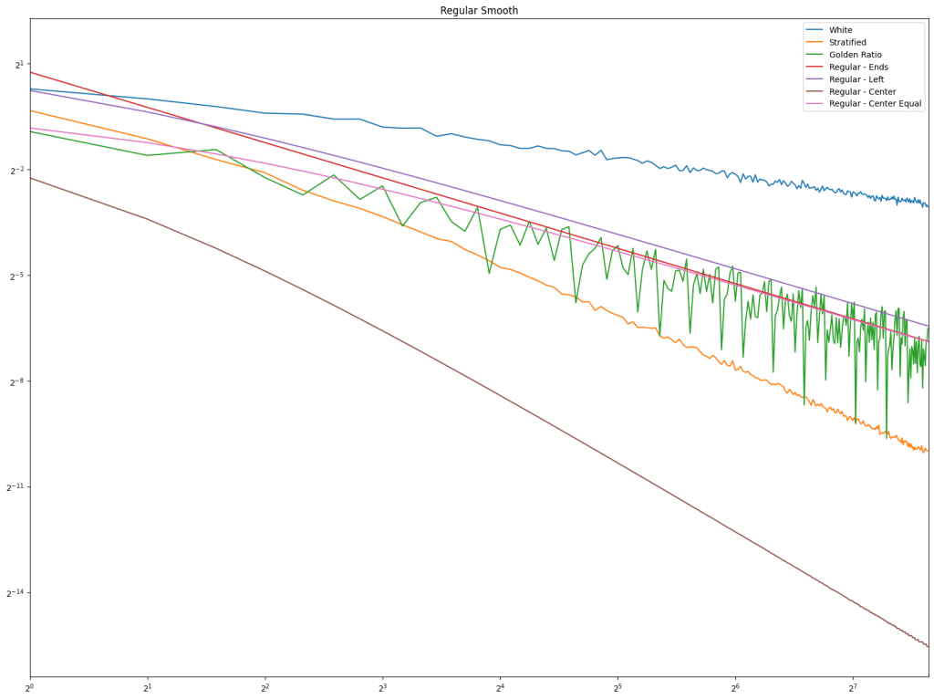
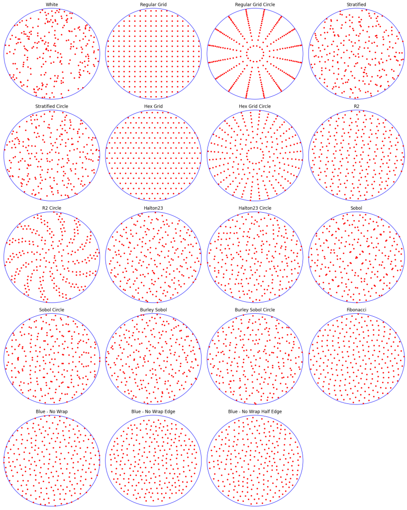
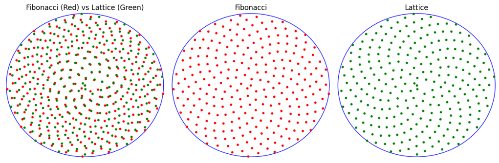
• Regular Grid Circle: “Regular center”, but x axis is multiplied by to make an angle, and y axis is square rooted to make a radius. This transformation maps a uniform random point in a square to a uniform random point in a circle and will be used by other sampling types too.
• Stratified: angle and radius as stratified.
• Stratified Circle: A stratified square is mapped to circle.
• Hex Grid: With rejection and filling in with white noise.
• Hex Grid Circle: Hex grid is mapped to circle
• R2: with rejection
• R2 Circle: R2 mapped to circle.
• Halton23: with rejection
• Halton23 Circle: mapped to circle
• Sobol: rejection
• Sobol Circle: mapped to circle
• Burley Sobol: rejection
• Burley Sobol Circle: mapped to circle
• Fibonacci: mapped to circle
• Blue No Wrap
• Blue No Wrap Edge
• Blue No Wrap Half Edge

The tests are the same as 2D square, but the functions are zero outside of a radius 0.5 circle.

Here are 256 samples of each.

Looking at regular sampling first. Fibonacci dominates but the regular sampling beats stratified.

Looking at LDS next, fibonacci does pretty well in a class by itself, except for the non smooth test where burley sobol joins it.

Lastly is blue noise which seems to indicate that wrapping would be good, by “half edge” distance doing the best for the most part. This is also showing that sampling away from the edges is a good thing.

Conclusion

Looking at sampling a 1D number line, a 2D square, and a 2D circle, regular sampling and blue noise have shown that avoiding the edge of the sampling domain by “half a point distance” (repel at half strength for blue noise) gives best results.

It makes me wonder though: why?

If you have any thoughts, hit me up on:

• Twitter: https://twitter.com/Atrix256
• Mastodon: https://mastodon.gamedev.place/@demofox

Fibonacci Looks Like a Rotated Grid, What Gives?

I got a good question on twitter after this post (https://twitter.com/Mtrl_Scientist/status/1644749290705649664?t=4MqnsDOpCSOwkfgvCqLXRw)

I don’t have much to say about why it looks like a rotated regular grid, but I can show how it’s different than one.

To do this, I grabbed 3 points of Fibonacci in a triangle, to get two vectors to use for lattice axes. I then used that to make a lattice that you can see below. Side by side Fibonacci and the lattice are hard to tell apart, but when they are put on top of each other, you can see how Fibonacci is not a lattice, but deviates from the lattice over space.

When we map it to a circle, the difference is more pronounced. The Fibonacci circle has that familiar look that you see in sunflowers. The Lattice however just looks like spirals. When they are overlaid, you can see they diverge quite a bit.

The C++ code that goes with this post is at https://github.com/Atrix256/EulersBestCandidate

The last post talked about links between Euler’s number e, and probability, inspired by a really cool youtube video on the subject: https://www.youtube.com/watch?v=AAir4vcxRPU

One of the things illustrated is that if you want to evaluate N candidates and pick the best one, you can evaluate the first N/e candidates (~36.8%), keep track of the highest score, then start evaluating the rest of the candidates, and choose the first one that scores higher.

That made me think of “Mitchell’s Best Candidate” algorithm for generating blue noise sample points. It isn’t the most modern way to make blue noise points, but it is easy to describe, easy to code, and gives decent-quality blue noise points.

I wrote up the algorithm in a previous blog post (https://blog.demofox.org/2017/10/20/generating-blue-noise-sample-points-with-mitchells-best-candidate-algorithm/) but here is a minimal description:

1. If you already have N blue noise points (N can be 0)
2. Generate N+1 white noise points as candidates.
3. The score for a candidate is the distance between it and the closest existing blue noise point.
4. Keep whichever candidate has the largest score.

The above generates one more blue noise point than you have. You repeat that until you have as many points as you want.

So, can we merge these two things? The idea is that instead of generating and evaluating all N+1 candidates, we generate and evaluate (N+1)/e of them, keeping track of the best score.

We then generate more candidates, until we find a candidate with a better score, and then exit, or until we run out of candidates, at which case we return the best candidate we found in the first (N+1)/e of them.

This is done through a simple modification in Mitchell’s Best Candidate algorithm:

1. We calculate a “minimum stopping index” which is ceil((N+1)/e).
2. When we are evaluating candidates, if we have a new best candidate, and the candidate index is >= the minimum stopping index, we exit the loop and stop generating and evaluating candidates.

Did it work? Here are two blue noise sets side by side. 1000 points each. Can you tell which is which?

Here are the averaged DFTs of 100 tests.

In both sets of images, the left is Mitchell’s Best Candidate, and the right is Euler’s Best Candidate.

The program output shows us that EBC took 71% of the time that MBC did though. Also, the inner most loop of these best candidate algorithms is calculating the distance between a candidate and an existing point. EBC only had to do 73.6% of these calculations as MBC did for the same quality result. While MBC has a fixed number of “hot loops”, EBC is randomized though and has a standard deviation of 3.5 million, when the operation takes at max 333 million, so has a standard deviation of about 1%.

It looks like a win to me! Note that the timing includes writing the noise to disk as pngs.

This could perhaps be a decent way to do randomized organic object placement on a map, like for bushes and trees and such. There are other algorithms that generate several candidates and keep the best one though. It should work just fine in those situations as well. Here is a mastodon thread on the subject https://mastodon.gamedev.place/@demofox/110030932447201035.

The next time you have to evaluate a bunch of random candidates to find the best one, you can remember “find the best out of the first 1/3, then continue processing til the next best one you find, or you run out of items”.

For more info, check out this Wikipedia page, which also talks about variations such as what to do if you don’t know how many candidates you are going to need: https://en.wikipedia.org/wiki/Secretary_problem

The source code that goes with this post can be found at https://github.com/Atrix256/EulerProbability

A few weeks ago I saw a great video on youtube that showed how Euler’s number e comes up everywhere.
https://www.youtube.com/watch?v=AAir4vcxRPU

It was a lot of the same old stuff we’ve all seen many times before but then started talking about Euler’s number showing up in probability. The video instantly had my full attention.

I spend a lot of time thinking about how uses of white noise can be turned into using blue noise or low discrepancy sequences because white noise has nice properties at the limit, but those other things have the same properties over much smaller numbers of samples. This link to probability made we wonder how other types of noise / sequences would behave when put through the same situations where Euler’s number emerged. Would e still emerge, or would it be a different value for different sequence types?

This is what sent me on the rabbit hole for the two prior blog posts, which explore making streaming uniform red noise, blue noise, and other random number generators.

Let’s get into it!

Lottery Winnings

One claim the video makes is that if the odds for winning the lottery are 1 in N, that if you buy N lottery tickets, there is a 1/e chance that you will still lose. 1/e is 0.367879, so that is a 36.79% of losing.

That may be true for white noise, but how about other sequences?

To test, I generate a random integer in [0,N) as the winning number, and then generate N more random numbers as the lottery tickets, each also in [0, N). The test results in a win (1) or a loss (0). This test is done 1,000,000 times to get an average chance of losing. Also, standard deviation is calculated by looking at the percentage of each group of 1,000 tests.

Here are the sequences tested:

• White Noise – regular old random numbers
• Golden Ratio – the deterministic golden ratio sequence: fract(index * phi)
• Stratified – stratify N buckets to make N numbers
• Regular Offset – N regularly spaced numbers, but with a random offset and modulus to keep them in range.
• Red Noise – made by adding two values together, converting from triangle to uniform, and rerolling one of the numbers for next time. Each number gets regenerated every other index. (https://blog.demofox.org/2023/02/20/uniform-1d-red-noise-blue-noise/)
• Blue Noise – made by subtracting one value from another, converting from triangle to uniform, and rerolling one of the numbers for next time. Each number gets regenerated every other index, and which value gets subtracted changes each index as well. (https://blog.demofox.org/2023/02/20/uniform-1d-red-noise-blue-noise/)
• Better Red Noise – FIR filtered white noise, with a piecewise polynomial to transform it back to uniform. (https://blog.demofox.org/2023/03/06/uniform-1d-red-noise-blue-noise-part-2/)
• Better Blue Noise – FIR filtered white noise, with a piecewise polynomial to transform it back to uniform. (https://blog.demofox.org/2023/03/06/uniform-1d-red-noise-blue-noise-part-2/)
• Better Blue Noise 2 – IIR filtering white noise, from Nick Appleton (https://blog.demofox.org/2023/03/06/uniform-1d-red-noise-blue-noise-part-2/)

We were able to duplicate the results for white noise which is neat. Using the golden ratio sequence cuts the loss rate in half. I chalk this up to it being more fairly distributed than white noise. White noise is going to give you the same lottery ticket number several times, where golden ratio is going to reduce that redundancy.

Stratified and regular offset both did very well on this test, but that isn’t surprising. If you have a 1 in N chance of picking a winning random number, and you make (almost) every number between 1 and N as a guess, you are going to (almost) always win. The little bit of randomization in each will keep them from winning 100% of the time.

the red noise and blue noise were very close to having a 1/e loss chance but were off in the tenths of a percentage place. Running it again gives similar results, so I think this could be a real, but small, effect. Colored noise seems like it affects this outcome a little bit.

Summing Random Values

Another claim the video makes is that if you add random uniform white noise numbers together, it will on average take e of them (2.718282) to be greater than or equal to 1. I do that test 100,000,000 times with each sequence again.

Let’s see:

We duplicated the results with white noise again, which is neat.

The golden ratio sequence takes slightly fewer numbers to reach 1.0. Subsequent numbers of the golden ratio sequence are pretty different usually, so this makes some sense to me.

For stratified and regular offset, I wanted to include them, but their sequence is in order, which doesn’t make sense for this test. So, I shuffled them. The result looks to be just a little bit lower than e.

The lower quality red and blue noise took quite a bit more numbers to reach 1.0 at 3.9 and 3.5 respectively. The better red noise took 3 numbers on average, while the blue noise took the lowest seen at 2.5 numbers. Lastly, the FIR blue noise “better blue noise 2” took just under e.

An interesting observation is that the red noises all have higher standard deviation than the other sequences. Red noise makes similar numbers consecutively, so if the numbers are smaller, it would take more of them, where if they were bigger it would take fewer of them. I think that is why the standard deviation (square root of variance) is higher. It’s just more erratic.

Contrary to that, the blue noise sequences have lower standard deviation. Blue noise makes dis-similar numbers consecutively, so I think it makes sense that it would be more consistent in how many numbers it took to sum to 1.0, and thus have a lower standard deviation and variance.

Finding The Best Scoring Item

The video also had this neat algorithm for fairly reliably finding the best scoring item, without having to look at all items.

Their setup is that you have job applicants to review and after talking to each, you have to decide right then to hire the person or to continue looking at other candidates. The algorithm is that you interview 1/e percent of them (36.79%), not hiring any of them, but keeping track of how well the best interviewer did. You then start interviewing the remaining candidates and hire the first one that does better than the previous best.

Doing this apparently gives you a 1/e (36.79%) chance of picking the actual best candidate, even though you don’t evaluate all the candidates. That is pretty neat.

I did this test 10,000,000 times for each sequence type

All sequence types looked at 733 or 734 candidates out of 1000 on average. The golden ratio sequence actually ended up looking at 755 on average though, and the better blue noise 2 sequence looked at 731. The standard deviation is ~243 for all of them, except for golden ratio which is 214. So… golden ratio looks at more candidates on average, but it’s also more consistent about the number of candidates it looks at.

Most sequence types had roughly 0.5 candidates on average better than the candidate hired. The golden ratio has 0.04 candidates better on average though. Red noise has slightly more candidates better than that though, at 0.6 and 0.73. The “Better Blue Noise 2” has a full 1.08 candidates better on average. The standard deviation follows these counts… golden ratio is the lowest standard deviation by far, red noise is higher than average, and the better blue noise 2 is much higher than the rest.

Closing

As usual, the lesson is that DSP, stochastic algorithms and sampling are deep topics.

Did I miss something, or is there something I should know? Leave a comment here or hit me up on mastodon at https://mastodon.gamedev.place/@demofox

The code that goes with this post can be found at https://github.com/Atrix256/ToUniform

My last blog post was on filtering a stream of uniform white noise to make a stream of red or blue noise, and then using the CDF (inverted inverse CDF) to transform the non uniform red or blue noise back into a uniform distribution while preserving the noise color. It is at https://blog.demofox.org/2023/02/20/uniform-1d-red-noise-blue-noise/

After that post, Bart commented:
https://mastodon.gamedev.place/@demofox/109909020853454095

That had me thinking about how you could make a CDF of any distribution, numerically. You could then store it in a LUT, or perhaps use least squares to fit a polynomial to the CDF.

I also got this interesting comment from Graeme.
https://mastodon.gamedev.place/@graeme/109916215756255970

I had never seen that before, only ever seeing that you can subtract a low pass filter from the identity filter to get a high pass filter (https://blog.demofox.org/2022/02/26/image-sharpening-convolution-kernels/). It made me want to check out that kind of a filter to see what the differences could be.

So, I started by generating 10 million values of white noise and then filtering it. I made a histogram of the results and divided the counts by 10 million to normalize it into a PDF. From there I made a CDF by making a table where each CDF bucket value was the sum of all PDF values with the same or lower index. From there I made a 1024 entry CDF table, as well as a smaller 64 entry one, and I also fit the CDF with piecewise polynomials (https://blog.demofox.org/2022/06/29/piecewise-least-squares-curve-fitting/).

With any of those 3 CDF approximations, I could filter white noise in the same way I did when generating the CDF, put the colored noise through the CDF function, and get out colored noise that was uniform distribution.

I wasn’t very happy with the results though. They were decent, but I felt like I was leaving some quality on the table. Going from real values to indices and back was a bit fiddly, even when getting the nuances correct. I mentioned that it was surprisingly hard to make a usable CDF from a histogram, and Nikita gave this great comment.

It took me a minute to understand but this is quite an amazing insight: If you generate a lot of numbers from an unknown PDF and sort them you now have a LUT of the inverse CDF! If you are wondering why that is such an exciting thing, give this a read https://blog.demofox.org/2017/08/05/generating-random-numbers-from-a-specific-distribution-by-inverting-the-cdf/.

The intuition here is that regions of values that are more probable will take up more indices and so if you randomly select an index, you are more likely to select from those regions.

So, if you have a black box that is giving you random numbers, you can generate random numbers from the same distribution just by storing a bunch of the numbers it gives you, sorting them, and using uniform random numbers to select items from that list. Better yet, select a random position between 0 and 1, multiply by the size of the list, and use linear interpolation between the indices when you get a fractional index.

Andrew Helmer let me know that this is called the “Empirical Distribution Function” (thanks!) https://en.wikipedia.org/wiki/Empirical_distribution_function

In our case where we are trying to make non uniform numbers be uniform again, we actually want the inverted inverse CDF, or in other words, we want the CDF. We can get a CDF value from the inverse CDF table by taking a value between 0 and 1 and finding where it occurs in the inverse CDF table. We’ll get a fractional index out if we use linear interpolation, and we can divide by the size of the array to get a value between 0 and 1. This is the CDF value for that input value. If we do this lookup for N evenly spaced values between 0 and 1, we can get a CDF look up table out.

I did that with a 1024 sized look up table, a 64 sized look up table, and I also fit a piecewise polynomial to the CDF, with piecewise least squares.

The results were improved! Fewer moving parts and fewer conversions. Nice.

I’ll show the results in a minute but here are the tests I did:

• Box 3 Red Noise: convolved the white noise with the kernel [1, 1, 1]
• Box 3 Blue Noise: convolved the white noise with the kernel [-1, 1, -1]. This is an unsharp mask because I subtracted the red noise kernel from [0,2,0].
• Box 5 Red Noise: [1,1,1,1,1]
• Box 5 Blue Noise 1: [-1, -1, 1, -1, -1]
• Box 5 Blue Noise 2: [1, -1, 1, -1, 1]
• Gauss 1.0 Blue Noise: A sigma 1 gaussian kernel, with alternating signs to make it a high pass filter [0.0002, -0.0060, 0.0606, -0.2417, 0.3829, -0.2417, 0.0606, -0.0060, 0.0002]. Kernel calculated from here http://demofox.org/gauss.html
• FIRHPF – a finite impulse response high pass filter. It’s just convolved with the kernel [0.5, -1.0, 0.5]. Kernel calculated from here http://demofox.org/DSPFIR/FIR.html/
• IIRHPF – an infinite impulse response high pass filter. It has the same “x coefficients” as the previous filter, but has a y coefficient of 0.9. Filter calculated from here http://demofox.org/DSPIIR/IIR.html.
• FIRLPF – the low pass filter version of FIRHPF. kernel [0.25, 0.5, 0.25]
• IIRLPF – the low pass filter version of IIRHPF. x coefficients are the same as the previous filter, but has a y coefficient of -0.9.
• Void And Cluster – I used the void and cluster algorithm to make 100,000 blue noise values, and I did this 100 times to get 10 million total blue noise values. There is a “seam” in the blue noise every 100,000 values but that shouldn’t be a big deal.
• Final BN LUT – I took the sized 64 CDF LUT from the FIRHPF test and used it to turn filtered white noise back to uniform.
• Final BN Polynomial – I took the 4 piecewise quadratic functions that fit the CDF of FIRHPF and used it to turn filtered white noise back to uniform.
• Final RN Polynomial – The filter from FIRLPF is used, along with the polynomial from the previous filter to make it uniform again. Luckily FIRLPF and IIRLPF have the same histogram and CDF, so can use the same polynomials!

CDFs

In the below, the blue line is the 4 piecewise quadratic functions fit to the CDF. The green dotted line is the size 1024 CDF table. The orange line is the size 64 CDF table.

For void and cluster, and the “Final BN” tests, the source values are uniform, so it doesn’t make much sense to make a CDF and convert them to uniform etc, but it wasn’t trivial to disable that testing for them.

Here is the error of the CDF approximations, using the size 1024 CDF LUT as the ground truth to calculate the error.

Frequencies (DFTs)

Here are the DFTs to show the frequencies in the streams of noise. Converting filtered white noise to uniform does change the frequency a bit, but looking at the low frequency magnitudes of void and cluster, that might just be part of the nature of uniform distributed colored noise. I’m not sure.

The blue line is the original values from E.g. filtering white noise. The other colors are when converting them to uniform.

Histograms

Here are the histograms, to see if they are appropriately uniform. The histograms come in sets of 4: the filtered noise, and then 3 methods for converting the filtered noise back to uniform. The graphs should be red from top to bottom, then left to right.

Streaming Blue Noise

Looking at the results, the FIRHPF results look pretty decent, with the polynomial fit having a better histogram than the size 64 CDF LUT. Only being a 3 tap filter means that it only needs to remember the last 2 “x values” that it has seen too, as a “delay line” for the FIR filter. Decent quality results and efficient to obtain. nice. The results of that are in the diagrams above as “Final BN Polynomial”.

I tried taking only the first half of the fits – either 32 of the 64 LUT entries, or only the first two of the four polynomials. For the second half of the curve, when x > 0.5, you set x to1-x, and the resulting y value gets flipped as 1-y too. I wasn’t getting great results though, even when adding a least squares constraint that CDF(0.5) = 0.5. I’m saving that battle for a future day. If you solve it though, leave a comment!

Below is the C++ code for streaming scalar valued blue noise – aka a blue noise PRNG. Also the same for red noise. The full source code can be found at https://github.com/Atrix256/ToUniform.

If you have a need of other colors of noise, of other histograms, hopefully, this post can help you achieve that.

class BlueNoiseStreamPolynomial
{
public:
	BlueNoiseStreamPolynomial(pcg32_random_t rng)
		: m_rng(rng)
	{
		m_lastValues[0] = RandomFloat01();
		m_lastValues[1] = RandomFloat01();
	}
	
	float Next()
	{
		// Filter uniform white noise to remove low frequencies and make it blue.
		// A side effect is the noise becomes non uniform.
		static const float xCoefficients[3] = {0.5f, -1.0f, 0.5f};

		float value = RandomFloat01();

		float y =
			value * xCoefficients[0] +
			m_lastValues[0] * xCoefficients[1] +
			m_lastValues[1] * xCoefficients[2];

		m_lastValues[1] = m_lastValues[0];
		m_lastValues[0] = value;

		// the noise is also [-1,1] now, normalize to [0,1]
		float x = y * 0.5f + 0.5f;

		// Make the noise uniform again by putting it through a piecewise cubic polynomial approximation of the CDF
		// Switched to Horner's method polynomials, and a polynomial array to avoid branching, per Marc Reynolds. Thanks!
		float polynomialCoefficients[16] = {
			5.25964f, 0.039474f, 0.000708779f, 0.0f,
			-5.20987f, 7.82905f, -1.93105f, 0.159677f,
			-5.22644f, 7.8272f, -1.91677f, 0.15507f,
			5.23882f, -15.761f, 15.8054f, -4.28323f
		};
		int first = std::min(int(x * 4.0f), 3) * 4;
		return polynomialCoefficients[first + 3] + x * (polynomialCoefficients[first + 2] + x * (polynomialCoefficients[first + 1] + x * polynomialCoefficients[first + 0]));
	}

private:
	float RandomFloat01()
	{
		// return a uniform white noise random float between 0 and 1.
		// Can use whatever RNG you want, such as std::mt19937.
		return ldexpf((float)pcg32_random_r(&m_rng), -32);
	}

	pcg32_random_t m_rng;
	float m_lastValues[2] = {};
};

class RedNoiseStreamPolynomial
{
public:
	RedNoiseStreamPolynomial(pcg32_random_t rng)
		: m_rng(rng)
	{
		m_lastValues[0] = RandomFloat01();
		m_lastValues[1] = RandomFloat01();
	}

	float Next()
	{
		// Filter uniform white noise to remove high frequencies and make it red.
		// A side effect is the noise becomes non uniform.
		static const float xCoefficients[3] = { 0.25f, 0.5f, 0.25f };

		float value = RandomFloat01();

		float y =
			value * xCoefficients[0] +
			m_lastValues[0] * xCoefficients[1] +
			m_lastValues[1] * xCoefficients[2];

		m_lastValues[1] = m_lastValues[0];
		m_lastValues[0] = value;

		float x = y;

		// Make the noise uniform again by putting it through a piecewise cubic polynomial approximation of the CDF
		// Switched to Horner's method polynomials, and a polynomial array to avoid branching, per Marc Reynolds. Thanks!
		float polynomialCoefficients[16] = {
			5.25964f, 0.039474f, 0.000708779f, 0.0f,
			-5.20987f, 7.82905f, -1.93105f, 0.159677f,
			-5.22644f, 7.8272f, -1.91677f, 0.15507f,
			5.23882f, -15.761f, 15.8054f, -4.28323f
		};
		int first = std::min(int(x * 4.0f), 3) * 4;
		return polynomialCoefficients[first + 3] + x * (polynomialCoefficients[first + 2] + x * (polynomialCoefficients[first + 1] + x * polynomialCoefficients[first + 0]));
	}

private:
	float RandomFloat01()
	{
		// return a uniform white noise random float between 0 and 1.
		// Can use whatever RNG you want, such as std::mt19937.
		return ldexpf((float)pcg32_random_r(&m_rng), -32);
	}

	pcg32_random_t m_rng;
	float m_lastValues[2] = {};
};

Update 3/12/23

Nick Appleton has another way to make streaming blue noise (https://mastodon.gamedev.place/@nickappleton/110012203119490715).

I coded it up and put it through my analysis so you could compare apples to apples. It looks pretty good!

Histograms

DFTs

Code

// From Nick Appleton:
// https://mastodon.gamedev.place/@nickappleton/110009300197779505
// But I'm using this for the single bit random value needed per number:
// https://blog.demofox.org/2013/07/07/a-super-tiny-random-number-generator/
// Which comes from:
// http://www.woodmann.com/forum/showthread.php?3100-super-tiny-PRNG
class BlueNoiseStreamAppleton
{
public:
	BlueNoiseStreamAppleton(unsigned int seed)
		: m_seed(seed)
		, m_p(0.0f)
	{
	}

	float Next()
	{
		float ret = (GenerateRandomBit() ? 1.0f : -1.0f) / 2.0f - m_p;
		m_p = ret / 2.0f;
		return ret;
	}

private:
	bool GenerateRandomBit()
	{
		m_seed += (m_seed * m_seed) | 5;
		return (m_seed & 0x80000000) != 0;
	}

	unsigned int m_seed;
	float m_p;
};

The code that generated the data for this post is at https://github.com/Atrix256/TriangleToUniform

A previous blog post talked about how DSP filtering can make noise of various colors: https://blog.demofox.org/2019/07/30/dice-distributions-noise-colors/

That noise was not uniformly distributed though. It was binomial, so ranged from triangular to Gaussian.

Another blog post talked about how to convert uniform random numbers into other distributions, by inverting the CDF: https://blog.demofox.org/2017/08/05/generating-random-numbers-from-a-specific-distribution-by-inverting-the-cdf/

Inverting the CDF lets you convert from uniform to non uniform distributions, but you can also use the CDF to convert from the non uniform distribution to a uniform distribution.

This means that just like you can square root a uniform random number between 0 and 1 to get a “linear” distributed random number where larger numbers are more likely, you could also take linear distributed random numbers and square them to get uniform random numbers.

float UniformToLinear(float x)
{
	// PDF In:  y = 1
	// PDF Out: y = 2x
	// ICDF:    y = sqrt(x)
	return std::sqrt(x);
}

float LinearToUniform(float x)
{
	// PDF In:  y = 2x
	// PDF Out: y = 1
	// ICDF:    y = x*x
	return x*x;
}

This can be useful when you use a two tap FIR filter which gives a triangle distribution out. You can adapt the LinearToUniform function to convert the first half of a triangle distribution back to uniform, the values between 0 and 0.5. For the second half of the triangle distribution, you can subtract it from 1.0, to get values between 0 and 0.5 again, convert from linear to uniform, and then subtract it from 1.0 again to flip it back around.

float TriangleToUniform(float x)
{
	if (x < 0.5f)
	{
		x = LinearToUniform(x * 2.0f) / 2.0f;
	}
	else
	{
		x = 1.0f - x;
		x = LinearToUniform(x * 2.0f) / 2.0f;
		x = 1.0f - x;
	}
	return x;
}

Let’s see how this works out in practice. In the first column below, it shows uniform being converted to linear and triangle, and back, to show that the round trip works.

In the second column, it shows red noise (low frequency random numbers) being made by adding two random numbers together, and then being made into uniform noise by converting from triangle to unfirom. It then also shows higher order red noise histograms.

The third column shows the same, but with blue noise (high frequency random numbers.

Here are the DFTs of the above, showing that the frequency content stays pretty similar through these various transformations.

So while we have the ability to convert 2 tap filtered noise from triangular distributed noise to uniform distributed noise, what about higher tap counts that give higher order binomial distributions?

It turns out the binomial quantile function (inverse CDF) doesn’t have a closed form that you can evaluate symbolically, which is unfortunate. Maybe two taps is good enough.

Here are some bread crumbs if you are interested in digging deeper
https://sigmoid.social/@demofox@mastodon.gamedev.place/109900303572389575
https://math.stackexchange.com/questions/2763270/quantile-function-for-binomial-distribution

Here are 20 values of each noise type to let you see what kind of values they actually have. The numbers are mapped to be between 0 and 1 even though these noise types naturally have other ranges. Order 2 red noise goes between 0 and 2 for example, and order 2 blue noise goes between -1 and 1.

Uniform
0.900403 0.246402 0.236748 0.057191 0.058894 0.434673 0.701137 0.261305 0.572679 0.643746 0.469458 0.77797 0.226739 0.181948 0.821556 0.661276 0.051249 0.769218 0.188764 0.43576

UniformToLinear
0.948896 0.496389 0.486568 0.239147 0.242681 0.659297 0.83734 0.51118 0.756755 0.802338 0.68517 0.882026 0.476172 0.426553 0.906397 0.813188 0.226382 0.877051 0.43447 0.660121

UniformToLinearToUniform
0.900403 0.246402 0.236748 0.057191 0.058894 0.434673 0.701137 0.261305 0.572679 0.643746 0.469458 0.77797 0.226739 0.181948 0.821556 0.661276 0.051249 0.769218 0.188764 0.43576

UniformToTriangle
0.776845 0.351 0.344056 0.169102 0.171601 0.466193 0.613437 0.361459 0.537766 0.577949 0.484488 0.666811 0.336704 0.301619 0.7013 0.588464 0.160076 0.660307 0.307216 0.466776

UniformToTriangleToUniform
0.900403 0.246402 0.236748 0.057191 0.058894 0.434673 0.701138 0.261305 0.572679 0.643746 0.469458 0.77797 0.226739 0.181948 0.821556 0.661276 0.051249 0.769218 0.188764 0.43576

order2RedNoise
0.321869 0.570975 0.546493 0.198164 0.559791 0.878273 0.800657 0.358752 0.356042 0.415941 0.459842 0.494419 0.215436 0.123045 0.267453 0.327641 0.485267 0.75219 0.67746 0.667561

order2RedNoiseToUniform
0.207199 0.631876 0.588662 0.078538 0.612432 0.970365 0.920525 0.257406 0.253531 0.346013 0.422909 0.4889 0.092826 0.03028 0.143062 0.214697 0.470969 0.877181 0.791936 0.778968

Order3RedNoise
0.335386 0.277424 0.53206 0.40188 0.502503 0.387789 0.390553 0.567394 0.547909 0.590254 0.429892 0.490403 0.391568 0.542284 0.545479 0.629202 0.582389 0.482149 0.442254 0.233653

Order4RedNoise
0.356291 0.356358 0.504111 0.503146 0.349194 0.316624 0.350564 0.329089 0.507805 0.555398 0.500458 0.643967 0.638761 0.659525 0.530838 0.450842 0.398863 0.407845 0.442873 0.324967

Order5RedNoise
0.595826 0.677254 0.591135 0.580018 0.482702 0.53669 0.367685 0.451726 0.454507 0.51374 0.631042 0.72763 0.538094 0.565055 0.51138 0.531387 0.568837 0.624056 0.469604 0.58843

order2BlueNoise
0.776161 0.416218 0.574676 0.125724 0.781581 0.530997 0.429622 0.484102 0.242817 0.766749 0.672426 0.275927 0.669314 0.290202 0.735534 0.523847 0.087859 0.822141 0.512319 0.419758

order2BlueNoiseToUniform
0.899792 0.346476 0.638198 0.031613 0.904586 0.560072 0.36915 0.46871 0.117921 0.891188 0.78539 0.152271 0.781293 0.168434 0.860115 0.546556 0.015438 0.936732 0.524335 0.352393

Order3BlueNoise
0.551499 0.366028 0.93273 0.481828 0.380887 0.495225 0.300059 0.51881 0.306799 0.356479 0.514701 0.498685 0.430205 0.573065 0.154976 0.667236 0.80882 0.616841 0.502323 0.426226

Order4BlueNoise
0.468794 0.473531 0.548515 0.461906 0.382252 0.692732 0.295499 0.523719 0.666799 0.415463 0.660763 0.362965 0.564584 0.371505 0.572822 0.494167 0.457531 0.420116 0.483063 0.526781

Order5BlueNoise
0.580763 0.461876 0.648067 0.466234 0.563966 0.455099 0.590905 0.252803 0.557458 0.306351 0.497475 0.618316 0.384632 0.56649 0.758528 0.412953 0.567208 0.330753 0.611306 0.330666

This post is the result of a collaboration between myself and R4 Unit on mastodon (https://mastodon.gamedev.place/@R4_Unit@sigmoid.social/109810895052157457). R4 Unit is actually the one who showed me you could animate blue noise textures by adding the golden ratio to each pixel value every frame too some years back 🙂

The code that goes with this post is at: https://github.com/Atrix256/GoldenRatio1DSorted

Golden Ratio or Fibonacci? Make up your mind!

Fibonacci and the golden ratio are often used interchangeably, which can be confusing but this is due to them being two sides of the same coin. If you divide a Fibonacci number by the previous Fibonacci number, you will get approximately the golden ratio 1.6180339887.

The first few Fibonacci numbers are

1, 1, 2, 3, 5, 8, 13, 21, 34, and 55

Starting at the second 1 and dividing each number by the last number gives

1, 2, 1.5, 1.666, 1.6, 1.625, 1.615, 1.619, and 1.6176

This converges to the golden ratio and is exactly the golden ratio at infinity.

The golden ratio appears as the greek letter “phi,” which rhymes with pi and pie. It looks like φ (lowercase) or ϕ (uppercase).

You’ll see circles talked about a lot in this post and might wonder why. In 1D sampling, we sample a function for x between 0 and 1. Our actual function might want us to sample a different domain (like say between 1 and 4), but for simplicity’s sake, we generate points between 0 and 1 and map them to the different values if needed. When generating low discrepancy sequences, we want to generate values between 0 and 1 through “some process.” When values outside 0 to 1 are generated, modulus brings them back in. It’s as if we rolled our 0 to 1 number line segment into a circle where 1 and 0 connect. A value of 1.5 goes around the circle 1.5 times and lands at the 0.5 mark. Our line segment is basically a circle.

You may wonder about the difference between a low discrepancy sequence and a low discrepancy set. A low discrepancy sequence is a sequence of points with an ordering, and Wikipedia states that any subsequence starting at the first index is also low discrepancy (https://en.wikipedia.org/wiki/Low-discrepancy_sequence). A low discrepancy set is a set of points where all points must be used before they are low discrepancy.

If you are wondering what low discrepancy means, discrepancy is a measurement of how evenly spaced the points are. Low discrepancy sequences have nearly evenly spaced points, but not quite. This is a valuable property for sampling, with one reason being that perfectly evenly spaced points are subject to aliasing. At the same time, completely random (uniform white noise) will form clumps and voids, have a high discrepancy, and leave parts of the sampling domain unsampled.

We’ll be talking about the golden ratio low discrepancy sequence next, which has an ordering and is low discrepancy at each step.

The Golden Ratio Low Discrepancy Sequence

The golden ratio low discrepancy sequence (LDS) is a 1D sampling sequence with some excellent properties. When viewing on a number line, or a circle, the following sample always appears in the largest gap. This is true no matter what index you start in the sequence, which is a bit of a mind-bender. See the animation below.

float GoldenRatioLDS(int index)
{
  return std::fmod(1.61803398875f * float(index), 1.0f);
}

Multiplying the index by the golden ratio will cause floating point inaccuracies that affect the sequence as the index gets larger, so it’s better to have a function that gives you the next value in the sequence, that you can call repeatedly.

We can realize we only care about the fractional part of the golden ratio and subtract one from it. This value is called the golden ratio conjugate and is the value of 1/φ, and it is every bit as irrational as the golden ratio.

For best results, you can supply a random floating point number between 0 and 1 as the first value in the sequence.

float GoldenRatioLDSNext(float last)
{
  return std::fmod(last + 0.61803398875f, 1.0f);
}

If you are using this in screen space or texel space, better results would be to use a blue noise texture as the source of the initial random value (https://blog.demofox.org/2020/05/10/ray-marching-fog-with-blue-noise/). If this is an animated image, even better results would be to use spatiotemporal blue noise for that (https://developer.nvidia.com/blog/rendering-in-real-time-with-spatiotemporal-blue-noise-textures-part-1/).

The golden ratio LDS has excellent convergence for 1D integration (* asterisk to be explained in next section), but the samples aren’t in a sorted order. Looking at the number line, you can see that the samples come in a somewhat random (progressive) order. If these sampling positions correspond to different places in memory, this is not great for memory caches.

Furthermore, some sampling algorithms require you to visit the sample points in a sorted order – for instance, when ray marching participating media and alpha compositing the samples to make the final result. Maybe it would be nice if they were in a sorted order?

For a deeper dive into the golden ratio and irrational numbers in sampling, give this a read: https://blog.demofox.org/2020/07/26/irrational-numbers/

Fibonacci Word Sampling

Wanting a sorted version of the golden ratio LDS, I tried to solve it myself at first. I analyzed the gaps between the numbers for different sample counts and found some interesting identities involving different powers of φ, 1/φ, and 1-1/φ. I found a pattern and was able to describe this as a binary sequence, with rules for how to split the binary sequence to get the next sample. Then I got stuck, unsure how to use this knowledge to make sample points in order.

I shared some tidbits, and R4 Unit asked what I was up to. After explaining, getting some great info back, having further conversations, and implementing in parallel, the solution came into focus.

Here are the ingredients:

1. The “Fibonacci Word” is similar to the rabbit sequence but connects to the golden ratio and the Fibonacci sequence. (https://en.wikipedia.org/wiki/Fibonacci_word)
2. If you divide a circle using the golden ratio, the smaller of the two angles made is called “The Golden Angle” (https://en.wikipedia.org/wiki/Golden_angle)
3. If you place marks on a circle at multiples of some number of degrees, there will ever be at most three distinct distances between points on the circle (https://en.wikipedia.org/wiki/Three-gap_theorem)
4. If using the golden angle, and a Fibonacci number of points, there are only ever two distances between points, and you can calculate them easily. Furthermore, if starting at a point on the circle, the “Infinite Fibonacci Word” will tell you the step size (0 = big, 1 = small) to take to get to the next point in the circle for the “Golden Angle Low Discrepancy Sequence.” See the bullet point here about unit circles and the golden angle sequence https://en.wikipedia.org/wiki/Fibonacci_word#Other_properties. We divide the sequence by 2pi to get 0 to 1 on a number line instead of 0 to 2pi as radians on a circle. The golden angle low discrepancy sequence is generated the same way as the golden ratio low discrepancy sequence but uses 0.38196601125 as the constant (2-φ, or 1/φ^2).
5. You can generate the Nth digit of the “Infinite Fibonacci Word” with a simple formula. (https://en.wikipedia.org/wiki/Fibonacci_word#Closed-form_expression_for_individual_digits)
6. You can start at any point of the circle. It just rotates the circle. That means that when we generate our sequence, we can start at any random point 0 to 1 as a randomizing offset, and the quality of the sequence is unaltered.

A naive implementation can be found at https://github.com/Atrix256/GoldenRatio1DSorted/blob/main/main.cpp in the SortedGoldenRatioSequenceTest() function. A much better implementation is in the function Sequence_FibonacciWord().

static const float c_goldenRatio = 1.61803398875f;
static const float c_goldenRatioConjugate = 0.61803398875f; // 1/goldenRatio or goldenRatio-1
 
float FibonacciWordSequenceNext(float last, float big, float small, float& run)
{
    run += c_goldenRatio;
    float shift = std::floor(run);
    run -= shift;
    return last + ((shift == 1.0f) ? small : big);
}
 
// big can be set to 1.0f / float(numSamples), but will return >= numSamples points if so.
std::vector<float> Sequence_FibonacciWord(float big)
{
    std::vector<float> ret;
    float small = big * c_goldenRatioConjugate;
    float run = c_goldenRatioConjugate;
    float sample = 0.0f;
    while (sample < 1.0f)
    {
        ret.push_back(sample);
        sample = FibonacciWordSequenceNext(sample, big, small, run);
    }
    return ret;
}

Generating the next sample is amazingly simple. If you print out the value of “shift,” you’ll see that it is the Infinite Fibonacci Word, which decides whether to add the small or large gap size to get to the next point.

Other Implementation Details

In practice, there is a challenge with this sampling sequence. If you ask for N samples, it will usually return slightly more samples than that.

You might think it’d be ok to truncate them and just throw out the extra ones. If you do that, your convergence will be bad due to areas not being sampled at the end of your sampling domain.

You may decide you could throw out the extra ones and renormalize the point set to span the 0 to 1 interval by stretching it out, even being careful to preserve the ratio of the gap at the end between the last sample and 1.0. Unfortunately, if you do that, your convergence is still bad.

I tried both things, and the convergence degraded such that it was no longer competitive. It was a no-go.

In the sample code, I tell it to generate N samples. If it comes back with too many, I decrement N and try again. This repeats until the right number of samples is returned, or going any lower would make me not have enough samples.

If there are too many samples at this point, I truncate and divide all samples by the first sample thrown away. This rescales the sequence to fill the full 0 to 1 domain.

This process makes the results used in the next section and is what I found to be best.

This is a very costly operation, speculatively generating sequences of unknown length in a loop until we get the right amount, but this is something that could be done in advance. You can know that if you want a specific N number of samples, you say to generate M samples instead and divide each sample by a constant k which is the sample that comes right after the last one.

This might be a pain and require a couple more shader constants or magic numbers, but consider it the cost of better convergence. The things we do for beauty!

One last item… when you implement this, you need a way to apply an offset to the sequence, using a blue noise texture or whatever else you might want to use. I had good luck multiplying my 0 to 1 random value by the number of indices in my sequence, and using the fractional part of the index as a multiplier of the either big or small sized gap for that index. It felt like that might not work well, because each index is either a large or small gap, and this treats them as the same size, but it didn’t damage the quality in my testing, so that was nice.

Convergence

Now that we can make the sequence, let’s see if it is any good.

I tested the usual choices for 1D integration against three functions, did this 10,000 times, and graphed the RMSE.

Sampling Types:

• Uniform – Uniform random white noise.
• RegularRandomOffset – Regularly spaced sampling (index/N), with a single global random offset added to all the samples to shift the sequence a random amount around the circle for each test.
• Stratified – Regular spaced sampling, but with a random offset added to each sample ((index + rand01()) / N).
• GoldenRatioRandomOffset – The golden ratio LDS, with a single global random offset added to all the samples to shift the sequence a random amount around the circle for each test.
• FibonacciWordRandomOffset – The sequence described in this post, with a single global random offset added to all the samples to shift the sequence a random amount around the circle for each test.

I also tested VanDerCorput base two and base three. Their results were similar to the golden ratio results and are unsorted so only cluttered the graph, and are thus omitted.

Sine: y = sin(pi * x)

Step: y = (x < 0.3) ? 1.0 : 0.0

Triangle: y = x

Well bummer… it turns out not to be so great vs stratified sampling or regular spaced sampling with a random global shift.

The power in the 1d golden ratio sequence is that for any number of samples you have, it is pretty good sampling, and you can add more to it. This is useful if you don’t know how many samples you are going to take, or if you want to have a good (progressive) result as you take more samples.

If you know how many samples you want, it looks like it’s better to go with stratified, or regularly spaced samples with a random global shift.

When I was early in this journey I made a typo in my code where it only tested N-1 samples in these convergence graphs instead of the full N samples. In that situation, golden ratio worked well because it works fine for any number of samples from 0 to M. The sorted golden ratio ended up working as well because it is “well spaced” for a fibonacci number of samples, but otherwise, the samples bunch up a little bit at the end, so removing the last sample wasn’t very damaging. Due to this unfortunate typo, I saw from early on that a sorted golden ratio sequence would be real valuable (like for ray marching fog volumes), to get better convergence while still being able to get samples in order.

This one didn’t work out, but oh well, onto the next thing 😛