In a previous post I showed how to use dual numbers to be able to get both the value and derivative of a function at the same time:
Dual Numbers & Automatic Differentiation
That post mentions that you can extend it to multivariable functions but doesn’t explain how. This post is that explanation, including simple working C++ code!
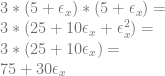
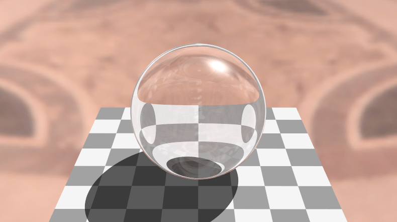
Extending this to multivariable functions is useful for ray marching, calculating analytical surface normals and also likely useful for training a neural network if you want an alternative to back propagation. I’m not sure about the efficiency comparison of this versus back propagation but I intend on looking into it (:
How Does it Work?
It turns out to be really simple to use dual numbers with multivariable functions. The end result is that you want a partial derivative for each variable in the equation, so to do that, you just have a dual number per variable, and process the entire equation for each of those dual numbers separately.
We’ll work through an example. Let’s find the partial derivatives of x and y of the function 
We’ll start by finding the derivative of x, and then the derivative of y.
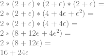
Example: df/dx
We start by making a dual number for our x value, remembering that the real part is the actual value for x, and the dual part is the derivative of x, which is 1:

or:

We multiply that value by itself to get the 


Next we need to multiply that by 3 to get the 

Putting that aside for a moment, we need to make the 

or:

If you are wondering why it has a zero for the epsilon term, it’s because when we are calculating the partial derivative of x, y is a constant, so has a derivative of zero.
Next, we multiply this y value by itself twice to get the 

We then multiply it by 2 to get the

Now that we have our two terms, we subtract the y term from the x term to get our final result:

This result says that
That checks out, let’s move on to the derivative of y!
Example: df/dy
Calculating the derivative of y is very similar to calculating the derivative of x, except that it’s the x term that has an epsilon value (derivative) of 0, instead of the y term. The y term has the epsilon value of 1 this time as well. We’ll work through it to see how it plays out.
First up, we need to make the value for x:

or:

Next we square it and multiply it by 3 to get the

Next we need to make the value for y, remembering that we use an epsilon value of 1 since the derivative of y is 1 this time around.

We cube that value and multiply by 2 to get the
Now we subtract the y term from the x term to get the final result:

This result says that
That also checks out, so we got the correct value and partial derivatives for the equation.
Reducing Redundancy
There was quite a bit of redundancy when working through the x and y derivatives wasn’t there? Increasing the number of variables will increase the amount of redundancy too, so it doesn’t scale up well.
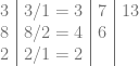
Luckily there is a way to address this. Basically, instead of making two dual numbers which have two items, you make them share the real value (since it’s the same for both, as is the work to make it) and append the dual values for x and y to it.
Thus, instead of having:

You have:
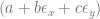
Then, in your math or in your program, you treat it as if it’s two different dual numbers packed into one. This lets you do the work for the real number once instead of twice, but still lets you do your dual number work for each variable independently.
While it’s probably easiest to think of these as two dual numbers packed into one value, there is actually a mathematical basis for it as well, which may or may not surprise you.
Check out what happens when we multiply two of these together, keeping in mind that multiplying ANY two epsilon values together becomes zero, even if they are different epsilons:

The interesting thing is that the above result gives you the same values as if you did the same work for two dual numbers individually.
Let’s see this three component dual number in action by re-doing the example again. Note that this pattern scales up to ANY number of variables!
Example: Both Derivatives (Gradient Vector)
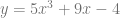
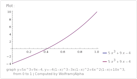
Our goal is to calculate the value and partial derivatives of the function
First we make our x value:

or:

We square that and multiply it by 3 to get our
Next, we make our y value:

or:

We cube it and multiply it by 2 to get our 

Lastly we subtract the y term from the x term to get our final answer:

The result says that
Neat, right?!
Example Code
Here is the example code output:

Here is the code that generated it:
#include <stdio.h>
#include <cmath>
#include <array>
#include <algorithm>

#define PI 3.14159265359f

#define EPSILON 0.001f  // for numeric derivatives calculation

template <size_t NUMVARIABLES>
class CDualNumber
{
public:

	// constructor to make a constant
	CDualNumber (float f = 0.0f) {
		m_real = f;
		std::fill(m_dual.begin(), m_dual.end(), 0.0f);
	}

	// constructor to make a variable value.  It sets the derivative to 1.0 for whichever variable this is a value for.
	CDualNumber (float f, size_t variableIndex) {
		m_real = f;
		std::fill(m_dual.begin(), m_dual.end(), 0.0f);
		m_dual[variableIndex] = 1.0f;
	}

	// storage for real and dual values
	float							m_real;
	std::array<float, NUMVARIABLES> m_dual;
};

//----------------------------------------------------------------------
// Math Operations
//----------------------------------------------------------------------
template <size_t NUMVARIABLES>
inline CDualNumber<NUMVARIABLES> operator + (const CDualNumber<NUMVARIABLES> &a, const CDualNumber<NUMVARIABLES> &b)
{
	CDualNumber<NUMVARIABLES> ret;
	ret.m_real = a.m_real + b.m_real;
	for (size_t i = 0; i < NUMVARIABLES; ++i)
		ret.m_dual[i] = a.m_dual[i] + b.m_dual[i];
	return ret;
}

template <size_t NUMVARIABLES>
inline CDualNumber<NUMVARIABLES> operator - (const CDualNumber<NUMVARIABLES> &a, const CDualNumber<NUMVARIABLES> &b)
{
	CDualNumber<NUMVARIABLES> ret;
	ret.m_real = a.m_real - b.m_real;
	for (size_t i = 0; i < NUMVARIABLES; ++i)
		ret.m_dual[i] = a.m_dual[i] - b.m_dual[i];
	return ret;
}

template <size_t NUMVARIABLES>
inline CDualNumber<NUMVARIABLES> operator * (const CDualNumber<NUMVARIABLES> &a, const CDualNumber<NUMVARIABLES> &b)
{
	CDualNumber<NUMVARIABLES> ret;
	ret.m_real = a.m_real * b.m_real;
	for (size_t i = 0; i < NUMVARIABLES; ++i)
		ret.m_dual[i] = a.m_real * b.m_dual[i] + a.m_dual[i] * b.m_real;
	return ret;
}

template <size_t NUMVARIABLES>
inline CDualNumber<NUMVARIABLES> operator / (const CDualNumber<NUMVARIABLES> &a, const CDualNumber<NUMVARIABLES> &b)
{
	CDualNumber<NUMVARIABLES> ret;
	ret.m_real = a.m_real / b.m_real;
	for (size_t i = 0; i < NUMVARIABLES; ++i)
		ret.m_dual[i] = (a.m_dual[i] * b.m_real - a.m_real * b.m_dual[i]) / (b.m_real * b.m_real);
	return ret;
}

template <size_t NUMVARIABLES>
inline CDualNumber<NUMVARIABLES> sqrt (const CDualNumber<NUMVARIABLES> &a)
{
	CDualNumber<NUMVARIABLES> ret;
	float sqrtReal = sqrt(a.m_real);
	ret.m_real = sqrtReal;
	for (size_t i = 0; i < NUMVARIABLES; ++i)
		ret.m_dual[i] = 0.5f * a.m_dual[i] / sqrtReal;
	return ret;
}

template <size_t NUMVARIABLES>
inline CDualNumber<NUMVARIABLES> pow (const CDualNumber<NUMVARIABLES> &a, float y)
{
	CDualNumber<NUMVARIABLES> ret;
	ret.m_real = pow(a.m_real, y);
	for (size_t i = 0; i < NUMVARIABLES; ++i)
		ret.m_dual[i] = y * a.m_dual[i] * pow(a.m_real, y - 1.0f);
	return ret;
}

template <size_t NUMVARIABLES>
inline CDualNumber<NUMVARIABLES> sin (const CDualNumber<NUMVARIABLES> &a)
{
	CDualNumber<NUMVARIABLES> ret;
	ret.m_real = sin(a.m_real);
	for (size_t i = 0; i < NUMVARIABLES; ++i)
		ret.m_dual[i] = a.m_dual[i] * cos(a.m_real);
	return ret;
}

template <size_t NUMVARIABLES>
inline CDualNumber<NUMVARIABLES> cos (const CDualNumber<NUMVARIABLES> &a)
{
	CDualNumber<NUMVARIABLES> ret;
	ret.m_real = cos(a.m_real);
	for (size_t i = 0; i < NUMVARIABLES; ++i)
		ret.m_dual[i] = -a.m_dual[i] * sin(a.m_real);
	return ret;
}

template <size_t NUMVARIABLES>
inline CDualNumber<NUMVARIABLES> tan (const CDualNumber<NUMVARIABLES> &a)
{
	CDualNumber<NUMVARIABLES> ret;
	ret.m_real = tan(a.m_real);
	for (size_t i = 0; i < NUMVARIABLES; ++i)
		ret.m_dual[i] = a.m_dual[i] / (cos(a.m_real) * cos(a.m_real));
	return ret;
}

template <size_t NUMVARIABLES>
inline CDualNumber<NUMVARIABLES> atan (const CDualNumber<NUMVARIABLES> &a)
{
	CDualNumber<NUMVARIABLES> ret;
	ret.m_real = tan(a.m_real);
	for (size_t i = 0; i < NUMVARIABLES; ++i)
		ret.m_dual[i] = a.m_dual[i] / (1.0f + a.m_real * a.m_real);
	return ret;
}

// templated so it can work for both a CDualNumber<1> and a float
template <typename T>
inline T SmoothStep (const T& x)
{
	return x * x * (T(3.0f) - T(2.0f) * x);
}

//----------------------------------------------------------------------
// Test Functions
//----------------------------------------------------------------------

void TestSmoothStep (float input)
{
	// create a dual number as the value of x
	CDualNumber<1> x(input, 0);

	// calculate value and derivative using dual numbers
	CDualNumber<1> y = SmoothStep(x);

	// calculate numeric derivative using central differences
	float derivNumeric = (SmoothStep(input + EPSILON) - SmoothStep(input - EPSILON)) / (2.0f * EPSILON);

	// calculate actual derivative
	float derivActual = 6.0f * input - 6.0f * input * input;

	// show value and derivatives
	printf("(smoothstep) y=3x^2-2x^3  (x=%0.4f)n", input);
	printf("  y = %0.4fn", y.m_real);
	printf("  dual# dy/dx = %0.4fn", y.m_dual[0]);
	printf("  actual dy/dx = %0.4fn", derivActual);
	printf("  numeric dy/dx = %0.4fnn", derivNumeric);
}

void TestTrig (float input)
{
	// create a dual number as the value of x
	CDualNumber<1> x(input, 0);

	// sin
	{
		// calculate value and derivative using dual numbers
		CDualNumber<1> y = sin(x);

		// calculate numeric derivative using central differences
		float derivNumeric = (sin(input + EPSILON) - sin(input - EPSILON)) / (2.0f * EPSILON);

		// calculate actual derivative
		float derivActual = cos(input);

		// show value and derivatives
		printf("sin(%0.4f) = %0.4fn", input, y.m_real);
		printf("  dual# dy/dx = %0.4fn", y.m_dual[0]);
		printf("  actual dy/dx = %0.4fn", derivActual);
		printf("  numeric dy/dx = %0.4fnn", derivNumeric);
	}

	// cos
	{
		// calculate value and derivative using dual numbers
		CDualNumber<1> y = cos(x);

		// calculate numeric derivative using central differences
		float derivNumeric = (cos(input + EPSILON) - cos(input - EPSILON)) / (2.0f * EPSILON);

		// calculate actual derivative
		float derivActual = -sin(input);

		// show value and derivatives
		printf("cos(%0.4f) = %0.4fn", input, y.m_real);
		printf("  dual# dy/dx = %0.4fn", y.m_dual[0]);
		printf("  actual dy/dx = %0.4fn", derivActual);
		printf("  numeric dy/dx = %0.4fnn", derivNumeric);
	}

	// tan
	{
		// calculate value and derivative using dual numbers
		CDualNumber<1> y = tan(x);

		// calculate numeric derivative using central differences
		float derivNumeric = (tan(input + EPSILON) - tan(input - EPSILON)) / (2.0f * EPSILON);

		// calculate actual derivative
		float derivActual = 1.0f / (cos(input)*cos(input));

		// show value and derivatives
		printf("tan(%0.4f) = %0.4fn", input, y.m_real);
		printf("  dual# dy/dx = %0.4fn", y.m_dual[0]);
		printf("  actual dy/dx = %0.4fn", derivActual);
		printf("  numeric dy/dx = %0.4fnn", derivNumeric);
	}

	// atan
	{
		// calculate value and derivative using dual numbers
		CDualNumber<1> y = atan(x);

		// calculate numeric derivative using central differences
		float derivNumeric = (atan(input + EPSILON) - atan(input - EPSILON)) / (2.0f * EPSILON);

		// calculate actual derivative
		float derivActual = 1.0f / (1.0f + input * input);

		// show value and derivatives
		printf("atan(%0.4f) = %0.4fn", input, y.m_real);
		printf("  dual# dy/dx = %0.4fn", y.m_dual[0]);
		printf("  actual dy/dx = %0.4fn", derivActual);
		printf("  numeric dy/dx = %0.4fnn", derivNumeric);
	}
}

void TestSimple (float input)
{
	// create a dual number as the value of x
	CDualNumber<1> x(input, 0);

	// sqrt
	{
		// calculate value and derivative using dual numbers
		CDualNumber<1> y = CDualNumber<1>(3.0f) / sqrt(x);

		// calculate numeric derivative using central differences
		float derivNumeric = ((3.0f / sqrt(input + EPSILON)) - (3.0f / sqrt(input - EPSILON))) / (2.0f * EPSILON);

		// calculate actual derivative
		float derivActual = -3.0f / (2.0f * pow(input, 3.0f / 2.0f));

		// show value and derivatives
		printf("3/sqrt(%0.4f) = %0.4fn", input, y.m_real);
		printf("  dual# dy/dx = %0.4fn", y.m_dual[0]);
		printf("  actual dy/dx = %0.4fn", derivActual);
		printf("  numeric dy/dx = %0.4fnn", derivNumeric);
	}

	// pow
	{
		// calculate value and derivative using dual numbers
		CDualNumber<1> y = pow(x + CDualNumber<1>(1.0f), 1.337f);

		// calculate numeric derivative using central differences
		float derivNumeric = ((pow(input + 1.0f + EPSILON, 1.337f)) - (pow(input + 1.0f - EPSILON, 1.337f))) / (2.0f * EPSILON);

		// calculate actual derivative
		float derivActual = 1.337f * pow(input + 1.0f, 0.337f);

		// show value and derivatives
		printf("(%0.4f+1)^1.337 = %0.4fn", input, y.m_real);
		printf("  dual# dy/dx = %0.4fn", y.m_dual[0]);
		printf("  actual dy/dx = %0.4fn", derivActual);
		printf("  numeric dy/dx = %0.4fnn", derivNumeric);
	}
}

void Test2D (float inputx, float inputy)
{
	// create dual numbers as the value of x and y
	CDualNumber<2> x(inputx, 0);
	CDualNumber<2> y(inputy, 1);

	// z = 3x^2 - 2y^3
	{
		// calculate value and partial derivatives using dual numbers
		CDualNumber<2> z = CDualNumber<2>(3.0f) * x * x - CDualNumber<2>(2.0f) * y * y * y;

		// calculate numeric partial derivatives using central differences
		auto f = [] (float x, float y) {
			return 3.0f * x * x - 2.0f * y * y * y;
		};
		float derivNumericX = (f(inputx + EPSILON, inputy) - f(inputx - EPSILON, inputy)) / (2.0f * EPSILON);
		float derivNumericY = (f(inputx, inputy + EPSILON) - f(inputx, inputy - EPSILON)) / (2.0f * EPSILON);

		// calculate actual partial derivatives
		float derivActualX = 6.0f * inputx;
		float derivActualY = -6.0f * inputy * inputy;

		// show value and derivatives
		printf("z=3x^2-2y^3 (x = %0.4f, y = %0.4f)n", inputx, inputy);
		printf("  z = %0.4fn", z.m_real);
		printf("  dual# dz/dx = %0.4fn", z.m_dual[0]);
		printf("  dual# dz/dy = %0.4fn", z.m_dual[1]);
		printf("  actual dz/dx = %0.4fn", derivActualX);
		printf("  actual dz/dy = %0.4fn", derivActualY);
		printf("  numeric dz/dx = %0.4fn", derivNumericX);
		printf("  numeric dz/dy = %0.4fnn", derivNumericY);
	}
}

void Test3D (float inputx, float inputy, float inputz)
{
	// create dual numbers as the value of x and y
	CDualNumber<3> x(inputx, 0);
	CDualNumber<3> y(inputy, 1);
	CDualNumber<3> z(inputz, 2);

	// w = sin(x*cos(2*y)) / tan(z)
	{
		// calculate value and partial derivatives using dual numbers
		CDualNumber<3> w = sin(x * cos(CDualNumber<3>(2.0f)*y)) / tan(z);

		// calculate numeric partial derivatives using central differences
		auto f = [] (float x, float y, float z) {
			return sin(x*cos(2.0f*y)) / tan(z);
		};
		float derivNumericX = (f(inputx + EPSILON, inputy, inputz) - f(inputx - EPSILON, inputy, inputz)) / (2.0f * EPSILON);
		float derivNumericY = (f(inputx, inputy + EPSILON, inputz) - f(inputx, inputy - EPSILON, inputz)) / (2.0f * EPSILON);
		float derivNumericZ = (f(inputx, inputy, inputz + EPSILON) - f(inputx, inputy, inputz - EPSILON)) / (2.0f * EPSILON);

		// calculate actual partial derivatives
		float derivActualX = cos(inputx*cos(2.0f*inputy))*cos(2.0f * inputy) / tan(inputz);
		float derivActualY = cos(inputx*cos(2.0f*inputy)) *-2.0f*inputx*sin(2.0f*inputy) / tan(inputz);
		float derivActualZ = sin(inputx * cos(2.0f * inputy)) / -(sin(inputz) * sin(inputz));

		// show value and derivatives
		printf("w=sin(x*cos(2*y))/tan(z) (x = %0.4f, y = %0.4f, z = %0.4f)n", inputx, inputy, inputz);
		printf("  w = %0.4fn", w.m_real);
		printf("  dual# dw/dx = %0.4fn", w.m_dual[0]);
		printf("  dual# dw/dy = %0.4fn", w.m_dual[1]);
		printf("  dual# dw/dz = %0.4fn", w.m_dual[2]);
		printf("  actual dw/dx = %0.4fn", derivActualX);
		printf("  actual dw/dy = %0.4fn", derivActualY);
		printf("  actual dw/dz = %0.4fn", derivActualZ);
		printf("  numeric dw/dx = %0.4fn", derivNumericX);
		printf("  numeric dw/dy = %0.4fn", derivNumericY);
		printf("  numeric dw/dz = %0.4fnn", derivNumericZ);
	}
}

int main (int argc, char **argv)
{
	TestSmoothStep(0.5f);
	TestSmoothStep(0.75f);
	TestTrig(PI * 0.25f);
	TestSimple(3.0f);
	Test2D(1.5f, 3.28f);
	Test3D(7.12f, 8.93f, 12.01f);
    return 0;
}
Closing
One of the neatest things about dual numbers is that they give precise results. They are not approximations and they are not numerical methods, unlike the central differences method that I compared them to in the example program (More info on numerical derivatives here: Finite Differences). Using dual numbers gives you exact derivatives, within the limitations of (eg) floating point math.
It turns out that backpropagation (the method that is commonly used to train neural networks) is just steepest gradient descent. You can read about that here: Backpropogation is Just Steepest Descent with Automatic Differentiation
That makes me wonder how dual numbers would do in run time speed compared to back propagation as well as numerical methods for getting the gradient to adjust a neural network during training.
If I had to guess, I’d say that dual numbers may be slightly slower than backpropagation, but not as slow as numerical methods which are going to be much, much slower. We’ll see though. It may be much easier to implement neural network learning using dual numbers compared to backpropagation, so may be worth an exploration and write up, even if only to make neural networks a little bit more accessible to people.
Comments, corrections, etc? Let me know in the comments below, or contact me on twitter at @Atrix256


 equation to a set of 2d data points, using least squares fitting. It allowed you to do this getting only one data point at a time, and still come up with the same answer as if you had all the data points at once, so it was an incremental, or “online” algorithm.
 ,
,  or greater.
 to calculate the coefficients (named c) of the equation.


 term, the next was for the
  term etc.

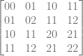

 has xy powers of 10. Permutation 0 has powers of 0,0 and permutation 2 has powers of 1,0, so we add those together to get powers 1,0.
 has xy powers of 21. Permutation 2 has powers of 1,0 and permutation 3 has powers 1,1. Adding those together we get 2,1 which is correct.


 or residue squared.
 .
.


 , where
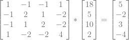
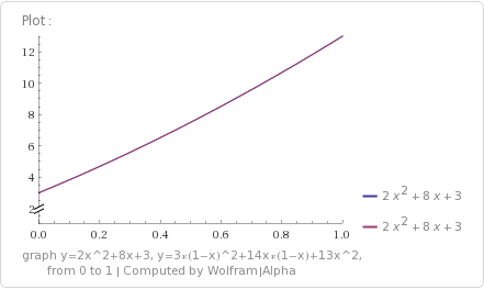
  and the matrix has NumDataPoints rows and Degree+1 columns. It looks like the below for a quadratic curve fitting 4 data points:

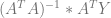
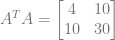
 , which we do below by multiplying the transpose of A by A:
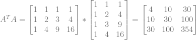
 . The inverse is:
 , which is the transpose of A multiplied by all of the Y values of our data:
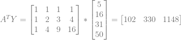
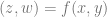
 :
:


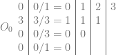
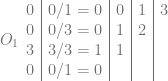
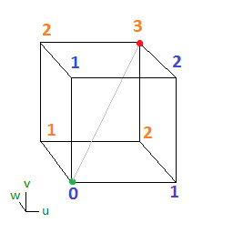
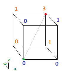
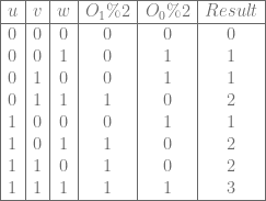
 will be the 1’s place output bit (least significant bit), and
  will be the 2’s place output bit (most significant bit). Our 3 input bits will be u,v,w.
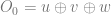

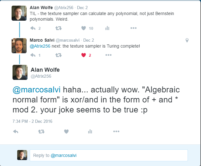
 ), and that XOR (
 ) is addition while AND is multiplication. This gives the formulas below:


 or
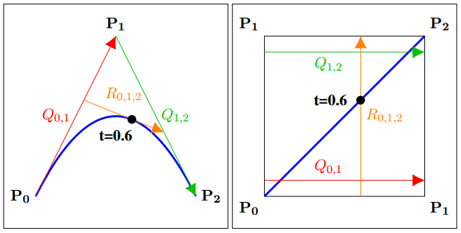
or  or by a constant or by another variable completely. My hope was that I’d be able to make the technique more generic and open it up to a larger family of equations, so people weren’t limited to just Bernstein polynomials.
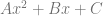 ) to “Bernstein Basis” (which looks like
  ) so long as they are the same degree.
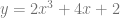 , that we can make this technique work for that too. The technique got a little closer to arbitrary equation evaluation. Neat!
 :
:


 instead of
  and also setting
  .
.


 at the front and the
  at the back) just means that we are going to take the result of everything between those two symbols, and add them up for every point in a hemisphere, multiplying each value by the fractional size of the point’s area for the hemisphere. The hemisphere we are talking about is the positive hemisphere surrounding the normal of the surface we are looking at.
 – This is the “Bidirectional reflectance distribution function”, otherwise known as the BRDF. It describes how much light is reflected towards the view direction, of the light coming in from the point on the hemisphere we are considering.
 – This is how much light is coming in from the point on the hemisphere we are considering.
 – This is the cosine of the angle between the point on the hemisphere we are considering and the surface normal, gotten via a dot product. What this term means is that as the light direction gets more perpendicular to the normal, light is reflected less and less. This is based on the actual behavior of light and you can read more about it here if you want to:


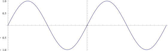
 samples of data, we multiply each sample of data by a sample from a wave with the frequency we are looking for and sum up the results (Note that this is really just a dot product between N dimensional vectors!). We have to do this both with a cosine wave and a sine wave, and keep the two resulting values to be able to get our true amplitude and phase information.


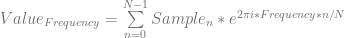

 is used instead of frequency.
 , the symbol is
  .
. , the symbol is
  .
.


 while a 2D Fourier transform is
  .
. time complexity.