Make sure and click the images in this post and view them at full size. Noise (especially blue noise) tends to disappear in smaller images.

There are 3 shadertoys that go with this post where you can see the techniques in action and see the source code of the implementations.

• Spherical Directional Light: https://www.shadertoy.com/view/3sfBWs
• Spherical Positional Light: https://www.shadertoy.com/view/ts2BRh
• Spherical Spot Light: https://www.shadertoy.com/view/tsjfRh

To go along with the blue noise ray marched fog and light shafts of the last post (Ray Marching Fog With Blue Noise), another fun usage case of blue noise is in raytracing soft shadows.

By soft shadows i mean the kinds of shadows you get from area lights, not the hard edged shadows you get from point lights and directional lights.

Soft shadows have a penumbra – the soft edges where it transitions from being fully in shadow to fully lit, like in the image below.

If you want to know more about why shadows work that way, give this post of mine a read: Why Are Some Shadows Soft And Other Shadows Hard?

So how do we use blue noise for this? We’re going to start with spherical directional lights first, then show how to extend it to spherical positional lights, and then to spherical spot lights.

Spherical Directional Light : White Noise

Shadertoy: https://www.shadertoy.com/view/3sfBWs

A directional light is a light that is shining from a specific direction, regardless of where you are at in the world.

These lights simulate light sources that are so far away, that any movement (translation) you do doesn’t measurably change your relative position to the light source because the sizes and distances involved are gigantic.

We are basically talking about the sun here.

Ok, so raytracing a shadow for a directional light like this just involves shooting a ray along the negative light direction (towards the sun) and seeing if it hits any geometry (the world, blocking the sun light). If it hits anything, the origin of the ray is in shadow. If it doesn’t hit anything, the origin of the ray is lit. The answer is binary and so the shadow edge is hard. There is no penumbra.

The problem with this model of lighting is that it pretends that the sun is an infinitely tiny point in the sky, when the sun is actually a circle, at least from our perspective. It is actually a sphere (or close enough to a sphere), but the “solid angle” 2d projection of it is a circle.

So, to have more realistic lighting and shadows, instead of shooting a ray at a single tiny point in space, we need to see if the ray origin can see the circle that is the spherical lighting source, and even more so, we need to know what percentage of the circle it can see.

The mathy explanation is we need to integrate visibility over the circle, but since our scene isn’t likely to be a closed form equation, we are going to need to resort to numerical methods and sample over the circle domain to get the shadow term.

The less mathy explanation is that we want to shoot rays at a couple places on that circle at random, and see what percentage of those rays were able to see the circle. We multiply the lighting by that percentage, and we automatically get soft shadows.

Ok so now that we know what we need to do, how do we do it?

So first up, we need to generate a “uniform point on a circle”, by which i mean generate a point where every point in the circle is equally likely to be chosen. If we have 2 uniform random numbers from 0 to 1 we can do that with the GLSL code below, assuming rng is a vec2 with two uniform random numbers in it. Any decent shader hash function or shader rng function should work for making those numbers, but i like using the “Hash without sine” functions from this shadertoy https://www.shadertoy.com/view/4djSRW

float pointRadius = c_lightRadius * sqrt(rng.x);
float pointAngle = rng.y * 2.0f * c_pi;
diskPoint = vec2(pointRadius*cos(pointAngle), pointRadius*sin(pointAngle));

Note c_lightRadius in the above. That value is the perceptual size of the circle in the sky. Like if you saw a photograph of the sky, this would be the radius of the circle of the sun if that photograph was 1 world unit away (the radius is in world space units under those strange viewing conditions). In the shadertoy demo I use a value of 0.1.

So now we have a uniform random point on a circle but what do we do with it? Well, to make it an actual point on the sun, we need a tangent basis so we have an X, Y and Z coordinate system to put this circle into.

Here is some GLSL to do that.

vec3 lightTangent = normalize(cross(c_lightDir, vec3(0.0f, 1.0f, 0.0f)));
vec3 lightBitangent = normalize(cross(lightTangent, c_lightDir));

This code assumes that the light direction is not ever going to point straight up. You could put in code to use a different vector if the light direction was ever too close to straight up if you want to fix that assumption. Also, c_lightDir is assumed to be normalized.

So now that we have a uniform random point on a circle, and we have a tangent basis aka coordinate system for that circle, it’s time to make a world space target for the ray to shoot at, so we can get a ray direction.

This part is pretty simple. We just pretend that the circle is 1 unit away and use the coordinate axes to convert the point on the circle into a world space point. From there, we subtract the ray’s position from the ray target position and normalize that vector, to get the ray direction.

vec3 rayTarget = rayPos + c_lightDir + diskPoint.x * lightTangent + diskPoint.y * lightBitangent;
vec3 shadowRayDir = normalize(rayTarget - rayPos);

Looking at that code, you might notice we are adding in the ray position, just to subtract it out again. We can skip a step and do this instead of the code above:

vec3 shadowRayDir = normalize(c_lightDir + diskPoint.x * lightTangent + diskPoint.y * lightBitangent);

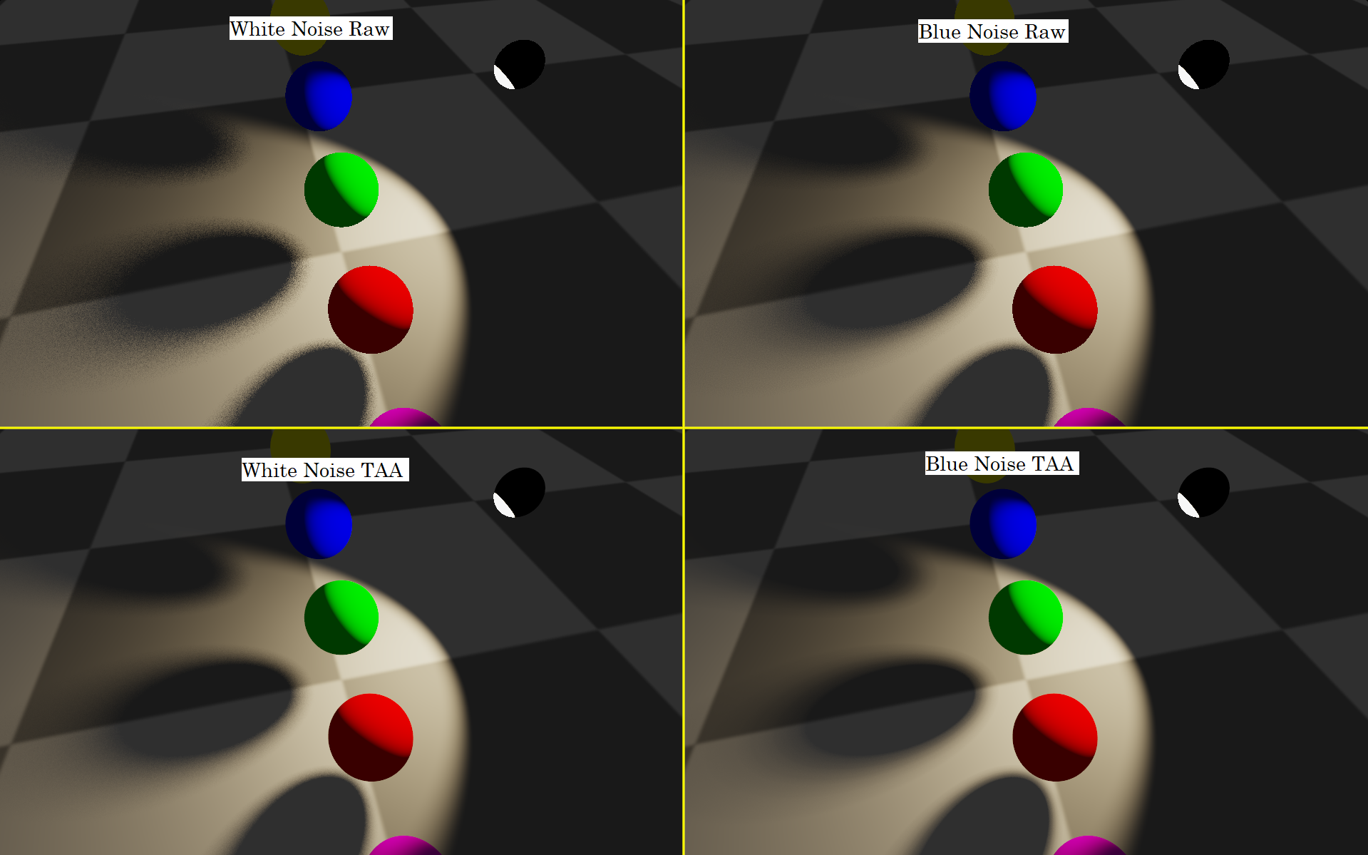
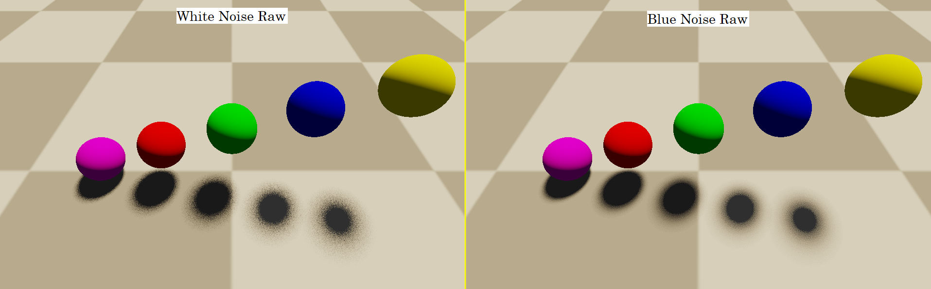
If you do this, you do in fact get a penumbra. This is what made the image labeled “white noise raw” in the image at the top of this section, using 16 shadow rays per pixel.

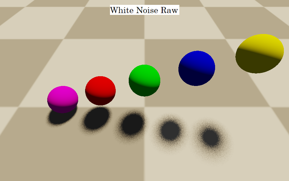
Quick note about perf: 16 shadow rays per pixel is kind of a lot. One way to help perf would be to say “if the first 4 rays all agree as to whether we are in shadow or not, just return that answer without doing the 12 other rays”. That would make this code cheaper everywhere except when in the penumbra. Another way to help perf would be to do shadows at a lower resolution. Another way would be to use fewer rays, but filter spatially and/or temporally (over time) to hide that fact. I’ve also heard of people making low resolution shadow maps and skipping the raytracing for pixels very clearly no where near a penumbra.

Spherical Directional Light : Blue Noise Over Space, Low Discrepancy Over Time

Being the blue noise zealot I am, white noise has a strong stink to me, and i know that if white noise is being used, almost certainly better results can be had by either using blue noise, or low discrepancy sequences instead.

We are actually going to use blue noise in 2 different ways to improve the shadows. The first way is that instead of using white noise (uncorrelated) uniform random numbers on the circle, we are going to use blue noise (negatively correlated) uniform random numbers on the circle.

White noise clumps together making semi redundant samples, and also leaves big holes between samples, making for larger unknown areas. Blue noise, on the other hand, is randomized, but roughly evenly spaced samples. (More info: What the heck is blue noise?)

I have some blue noise in a circle points i generated by using mitchell’s best candidate algorithm, but when generating candidates, i made sure they were all in a circle before doing the rest of the logic (aka i used rejection sampling inside of MBC). I also made it not calculate distances toroidally, since wrap around doesn’t make sense in this context. The points are also generated in [-1,1] instead of the usual [0,1].

For details of Mitchell’s best candidate algorithm check out my blog post: Generating Blue Noise Sample Points With Mitchell’s Best Candidate Algorithm

Below is that list of points I generated. These blue noise points are progressive, meaning that if you use the first N, regardless of what N is, you will have blue noise. So, this supports up to 64 samples, or any lower number of samples.

const vec2 BlueNoiseInDisk[64] = vec2[64](
    vec2(0.478712,0.875764),
    vec2(-0.337956,-0.793959),
    vec2(-0.955259,-0.028164),
    vec2(0.864527,0.325689),
    vec2(0.209342,-0.395657),
    vec2(-0.106779,0.672585),
    vec2(0.156213,0.235113),
    vec2(-0.413644,-0.082856),
    vec2(-0.415667,0.323909),
    vec2(0.141896,-0.939980),
    vec2(0.954932,-0.182516),
    vec2(-0.766184,0.410799),
    vec2(-0.434912,-0.458845),
    vec2(0.415242,-0.078724),
    vec2(0.728335,-0.491777),
    vec2(-0.058086,-0.066401),
    vec2(0.202990,0.686837),
    vec2(-0.808362,-0.556402),
    vec2(0.507386,-0.640839),
    vec2(-0.723494,-0.229240),
    vec2(0.489740,0.317826),
    vec2(-0.622663,0.765301),
    vec2(-0.010640,0.929347),
    vec2(0.663146,0.647618),
    vec2(-0.096674,-0.413835),
    vec2(0.525945,-0.321063),
    vec2(-0.122533,0.366019),
    vec2(0.195235,-0.687983),
    vec2(-0.563203,0.098748),
    vec2(0.418563,0.561335),
    vec2(-0.378595,0.800367),
    vec2(0.826922,0.001024),
    vec2(-0.085372,-0.766651),
    vec2(-0.921920,0.183673),
    vec2(-0.590008,-0.721799),
    vec2(0.167751,-0.164393),
    vec2(0.032961,-0.562530),
    vec2(0.632900,-0.107059),
    vec2(-0.464080,0.569669),
    vec2(-0.173676,-0.958758),
    vec2(-0.242648,-0.234303),
    vec2(-0.275362,0.157163),
    vec2(0.382295,-0.795131),
    vec2(0.562955,0.115562),
    vec2(0.190586,0.470121),
    vec2(0.770764,-0.297576),
    vec2(0.237281,0.931050),
    vec2(-0.666642,-0.455871),
    vec2(-0.905649,-0.298379),
    vec2(0.339520,0.157829),
    vec2(0.701438,-0.704100),
    vec2(-0.062758,0.160346),
    vec2(-0.220674,0.957141),
    vec2(0.642692,0.432706),
    vec2(-0.773390,-0.015272),
    vec2(-0.671467,0.246880),
    vec2(0.158051,0.062859),
    vec2(0.806009,0.527232),
    vec2(-0.057620,-0.247071),
    vec2(0.333436,-0.516710),
    vec2(-0.550658,-0.315773),
    vec2(-0.652078,0.589846),
    vec2(0.008818,0.530556),
    vec2(-0.210004,0.519896) 
);

Just doing that change, we get this strange result:

The problem is that every pixel is using the same blue noise sample sequence, and there are only 16 samples. That means there are 16 overlapping shadows for each sphere basically. Blue noise has done a good job in that those shadows are pretty different from each other, but the shadows aren’t good enough yet.

Now we need to bring in the second blue noise. We are going to tile a blue noise texture in screen space (you can get one here: http://momentsingraphics.de/BlueNoise.html), so that we can get a “blue noise random value” per pixel that is between 0 and 1. We are going to multiply that value by 2 * pi and use that as an angle for how to rotate our 2d blue noise samples.

Each pixel will have a different rotation amount, and each pixel will use a rotation that is very different from the rotation of neighboring pixels. This is due to blue noise textures having that property: pixel values are very different from neighbor pixel values.

A nice optimization here is that since all samples are being rotated by the same amount for a pixel, you can calculate the cosine and sine of the angle outside of the loop for shooting shadow rays, and just re-use them inside that loop for rotation.

If we do that, we end up with the image on the right labeled “blue noise raw”. Compare it vs “white noise raw” to see how the noise in the penumbra is way less noticeable. Same number of samples, same amount of computational complexity.

We aren’t done yet though… we have to now consider the axis of time, before we can declare victory.

Cutting right to the case, we are going to add frameNumber * goldenRatio to the blue noise value and fract it to bring it back to the 0 to 1 range. We want to do that before we multiply by 2 * pi to make it an angle.

If we do that, the blue noise value for each pixel becomes a low discrepancy sequence over time. It damages our blue noise over space property a little but it is a net win.

For a deeper discussion about this topic, check out these posts:
Animating Noise For Integration Over Time
Animating Noise For Integration Over Time 2: Uniform Over Time

The short answer to why this is better is that the distribution of a pixel’s value over time for shorter time durations is going to be closer to the actual distribution of the pixel. This is in contrast to white noise which does have the right average over larger sample counts, but for shorter sample counts may clump values together, and leave voids of unseen values.

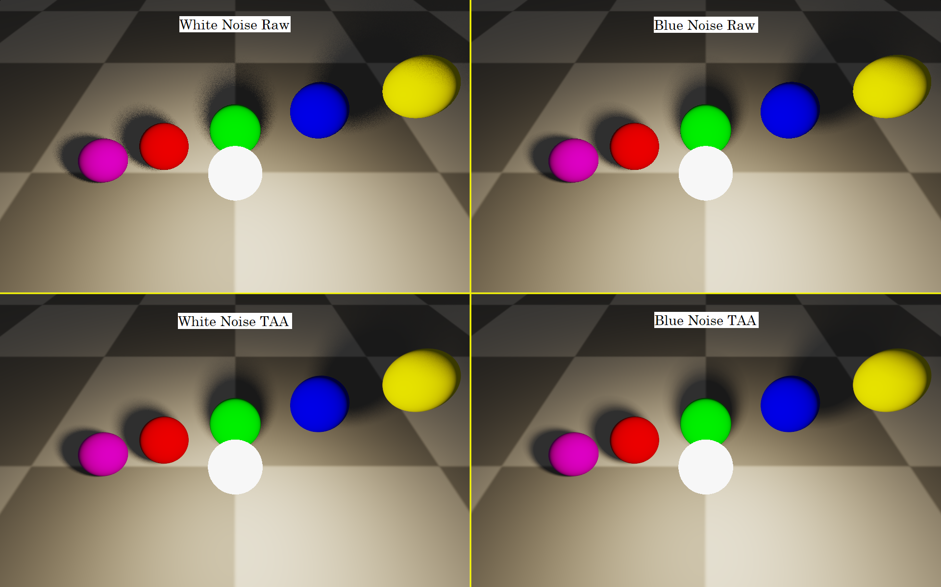
In short, this makes the pixel more temporally stable, which is great for TAA and other temporal filtering/accumulation methods, but also is nicer even when viewing it without temporal filtering. You can turn on and off the ANIMATE_NOISE define in the shader and look at the “blue noise raw” panel to see how it looks when animated vs not animated without filtering.

Here are the final results, and the link to the shadertoy again.

Shadertoy: https://www.shadertoy.com/view/3sfBWs

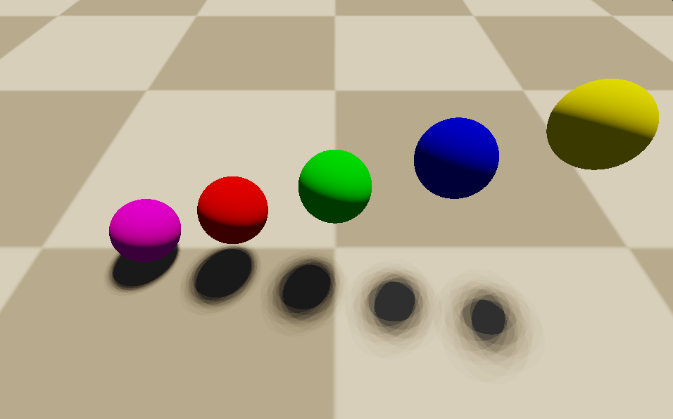
By the way, noise is way more noticeable when it’s high contrast with the things around it. For instance, here’s the same image as the above again, but the ambient lighting is 10 times brighter (0.5, instead of 0.05). It’s way harder to see the noise, even the white noise!

Spherical Positional Light

With spherical directional lights explained, the hard part is done!

You only need to make 2 modifications to your code to get from spherical directional lights to spherical positional lights.

The first change is that instead of c_lightDir being a constant, wherever you use that vector, you should instead use the normalized vector pointing from the pixel being shaded to the position of the light (the center of the light).

The second change is that c_lightRadius isn’t constant either anymore. Unlike the sun, which doesn’t noticeably change size as you move around the world, spherical positional lights DO noticeably change size. As you get farther away from the light, the 2d projected circle for that light gets smaller. As you get closer, the circle gets larger.

The formula is actually real simple. If c_lightRadius is the radius of the sphere, and dist is the distance from the shaded pixel to the center of the light, the actual radius you should use for the circle when doing the rest of the “spherical directional light” logic is just: c_lightRadius / dist.

Making those changes, you can get this:

Shadertoy: https://www.shadertoy.com/view/ts2BRh

Spherical Spot Light

Now that you have a spherical positional light, it’s pretty easy to modify it into a spherical spotlight.

The first thing to do is to re-introduce a light direction. This light direction is the direction that the spot light is shining in. We are going to dot product the vector from the light to the pixel by this light direction to know what angle the pixel is from the light, to know if it’s in the light cone of the spot light or not.

The next thing to do is to define a “cosine theta inner” and a “cosine theta outer”. When the dot product in the last paragraph is less than “cosine theta outer”, then there is no light. If it’s greater than “cosine theta inner” then it’s full light. Between those values we want it to fade from lit to unlit, and for that i like to use smoothstep to do a non linear fade. Here’s some glsl code that does this:

vec3 lightDir = normalize(c_lightPos - hitPos);
float angleAtten = dot(lightDir, -c_lightDir);
angleAtten = smoothstep(c_cosThetaOuter, c_cosThetaInner, angleAtten);
lightColor *= angleAtten;

The rest of the code runs the same as a Spherical Positional Light, and you get a result like this:

Shadertoy: https://www.shadertoy.com/view/tsjfRh

Summary

This post showed how to use blue noise in two different ways for raytracing soft shadows.

1. Blue noise sample points in a circle were used to sample a circle representing the light. Using blue noise here results in less error than white noise.
2. A blue noise texture was used to rotate those 2d sample points per each pixel to make the resulting error be screen space blue noise, which looks better, is harder to detect, and is filtered more easily, compared to white noise, even for the same amount of error.

An important note here is that while blue noise converges at the same rate as white noise (but starts with lower error), low discrepancy sequences can converge quite a bit faster than white noise or blue noise.

If we could use a low discrepancy sequence for sampling the circle in step 1 above and converge so that there was no error, we could be done and wouldn’t need to do step 2.

Unfortunately, low discrepancy sequences have aliasing and so have worse looking error than blue noise before they converge. For the ray sample counts we have in budget right now for real time rendering, we definitely can’t afford to converge, even with an LDS, so that is why we reached for blue noise.

This is important to know, because for non real time rendering usage cases, you are likely better off with an LDS, than blue noise. Blue noise is just a neat trick you can do when you are really strapped for samples (aka can’t afford many rays).

One last thing – it turns out that sampling the projected 2d circle for 3d spherical lights is not quite the correct thing to do. It’s a decent approximation but for more information, check out this link (and note, you can apply blue noise the same way with better spherical light sampling):

https://schuttejoe.github.io/post/arealightsampling/

Happy raytracing and feel free to hit me up on shadertoy or on twitter if you have any questions @Atrix256